
Table of Contents
Oscillator Technical Indicator is a technical indicator used in the financial market analysis for assessing the over-bought/over-sold of a given asset in a given period. It can assist investors in identifying trends and potential trend reversals.
Oscillator Technical Indicator processes and converts specific price indicators (e.g., opening, closing, highest, and lowest price) in a limited range. Some may include a negative range. Oscillator Technical Indicators are normally presented in a linear format.
Today, we are going to introduce an Oscillator Technical Indicator — Aroon Up Down.
Aroon Indicator, developed by Tushar Chande in 1995, is typically for measuring market tendency. It consists of two lines - Aroon Up and Aroon Down.
Aroon Up:((Number of periods - Number of periods since highest high) / Number of periods) * 100
This indicator measures the periods since the highest price (high point) occurred within the selected period.
Aroon Down:((Number of periods - Number of periods since lowest low) / Number of periods) * 100
This indicator measures the periods since the lowest price (low point) occurred within the selected period.
The Aroon Up indicator measures the strength and time since the highest price within a given period (usually 25 periods). In contrast, the Aroon Down indicator measures the strength and time since the lowest price within the same period. These indicators are expressed as percentages and range from 0% to 100%.
The crossover of the Aroon Up and Aroon Down lines can be used to signal potential changes in trend direction. For example, when Aroon Up crosses above Aroon Down, it might be seen as a bullish signal, indicating a potential shift towards an upward trend. Conversely, when Aroon Down crosses above Aroon Up, it could be interpreted as a bearish signal, suggesting a potential shift towards a downward trend.
MacOS and Jupyter Notebook is used as editor
import pandas as pd
import re
import numpy as np
import tejapi
import plotly.express as px
import matplotlib.pyplot as plt
import matplotlib.ticker as mticker
from matplotlib.pyplot import MultipleLocator
from sklearn.linear_model import LinearRegression
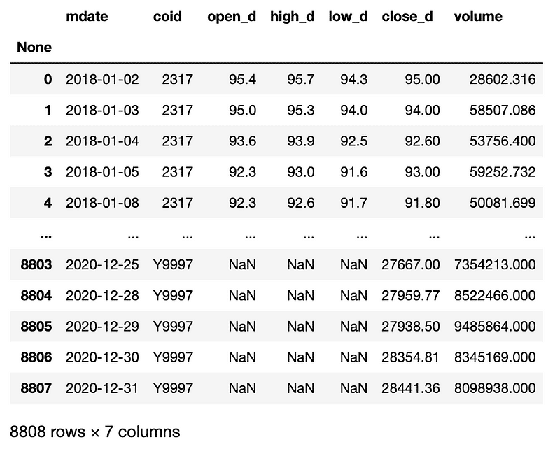
import datetimeFor the period from 2018–01–01 to 2020–12–31, we take Hon Hai Precision Industry Co., Ltd.(2317), Compal Electronics, Inc.(2324), YAGEO Corporation(2327), Taiwan Semiconductor Manufacturing Co., Ltd.(2330), Synnex Technology International Corp.(2347), Acer(2353), Foxconn Technology Co., Ltd.(2354), ASUS(2357), Realtek Semiconductor Corp.(2379), Quanta Computer, Inc.(2382), Advantech Co., Ltd.(2395) as instances, we will construct backtesting system with unadjusted price data, and compare the performance with the Market Return Index(Y9997).
stock_id = ["Y9997", "2317", "2324", "2327", "2330", "2347", "2353", "2354",
            "2357", "2379", "2382", "2395"]
gte, lte = '2018-01-01', '2020-12-31'
stock = tejapi.get('TWN/APRCD',
                   paginate = True,
                   coid = stock_id,
                   mdate = {'gte':gte, 'lte':lte},
                   opts = {
                       'columns':[ 'mdate', 'coid', 'open_d', 'high_d', 'low_d', 'close_d', 'volume']
                   }
                  )
Next, we transfer the table to the pivot table by coid(company id) and exclude the market index.
data_pivot = pd.pivot_table(stock[stock.coid != "Y9997"], columns="coid", index="mdate")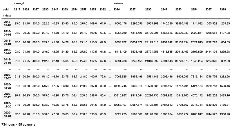
First of all, we need to declare the following arguments:
Because today’s demo is a multi-target trading strategy, we will use for loop to create a dictionary to retain the following info:
We use a list type object aroon_record to record each target’s “coid”, “mdate”, “Aroon-up”, “Aroon-down”.
Besides, to measure the eventual performance of our portfolio, we create two list-type objects - daily_stock_value_record and daily_cash_value_record to store each transaction day’s “holding position,” “stock value,” and “remaining cash value.”
Now, it’s time to design our trading signals.
When Aroon Up is greater than 80 and Aroon Down is lesser than 45, which represents a bullish trend. We consider it a buying signal and will acquire one unit at tomorrow’s opening price.
When Aroon Up is lesser than 45, Aroon Down is greater than 55, and the gap of two indicators is greater than 15, we regard it as a selling signal and sell the holding position at tomorrow’s opening price.
When Aroon Up is greater than 55, Aroon Down is lesser 45, the gap between the two indicators is greater than 15, our invested amount isn’t greater than 20% principal, and we still have plentiful cash. We will acquire one more unit at tomorrow’s opening price.
def Aroon_strategy_multi(data_pivot, principal, cash, order_unit, n):
    trade_book = pd.DataFrame()
    aroon = pd.DataFrame(columns=["coid", "mdate", "AroonUp", "AroonDown"])

    daily_stock_value_record = []
    daily_cash_value_record = []

    coid_dict = {}
    for i in list(data_pivot.high_d.columns):
        coid_dict.update({i:{"position":0, "invested_principal":0}})

    for ind in range(len(data_pivot.index) - n -1):
        for col in data_pivot.high_d.columns:
            high_period = data_pivot.high_d[col].iloc[ ind : ind+n].reset_index()
            AroonUp = round((high_period.idxmax()[1] + 1)/n*100)

            low_period = data_pivot.low_d[col].iloc[ ind : ind+n].reset_index()
            AroonDown = round(((low_period.idxmin()[1] + 1)/n*100))


            aroon = aroon.append({
                "coid":col,
                "mdate":data_pivot.index[ind+n],
                "AroonUp":AroonUp,
                "AroonDown":AroonDown,
            }, ignore_index=True)

            n_time = data_pivot.index[ind+n+1]
            n_open = data_pivot.open_d[col].iloc[ind+n+1]


            if coid_dict.get(col).get("position") == 0: #進場條件
                if (AroonDown < 45) and (AroonUp > 80):
                    position = coid_dict.get(col).get("position")

                    order_time = n_time
                    order_price = n_open
                    order_unit = 1
                    friction_cost = (20 if order_price*1000*0.001425 < 20 else order_price*1000*0.001425)
                    total_cost = -1 * order_price * 1000 - friction_cost
                    cash += total_cost

                    coid_dict.update({col:{"position":position+1, "invested_principal":order_price * 1000,}})

                    trade_book = pd.concat([trade_book,
                                           pd.DataFrame([col, 'Buy', order_time, 0,  total_cost, order_unit, coid_dict.get(col).get("position"), cash, order_price])],
                                           ignore_index = True, axis=1)

            elif coid_dict.get(col).get("position") > 0:
                if (AroonDown - AroonUp) > 15 and AroonDown > 55 and AroonUp < 45: # 出場條件
                    order_unit = coid_dict.get(col).get("position")
                    cover_time = n_time
                    cover_price = n_open
                    friction_cost = (20 if cover_price*order_unit*1000*0.001425 < 20 else cover_price*order_unit*1000*0.001425) + cover_price*order_unit*1000*0.003
                    total_cost = cover_price*order_unit*1000-friction_cost
                    cash += total_cost

                    coid_dict.update({col:{"position":0, "invested_principal":0}})

                    trade_book = pd.concat([trade_book,
                                           pd.DataFrame([col, 'Sell', 0, cover_time,  total_cost, -1*order_unit, coid_dict.get(col).get("position"), cash, cover_price])],
                                           ignore_index = True, axis=1)

                elif (AroonUp - AroonDown) > 15 and (AroonDown < 45) and AroonUp > 55 and (cash >= n_open*1000) and (coid_dict.get(col).get("invested_principal") <= 0.2 * principal): #加碼條件
                    order_unit = 1
                    order_time = n_time
                    order_price = n_open

                    position = coid_dict.get(col).get("position")

                    friction_cost = (20 if order_price*1000*0.001425 < 20 else order_price*1000*0.001425)
                    total_cost = -1 * order_price * 1000 - friction_cost
                    cash += total_cost

                    invested_principal = coid_dict.get(col).get("invested_principal")
                    coid_dict.update({col:{"position":position+1, "invested_principal": invested_principal + order_price*1000}})

                    trade_book = pd.concat([trade_book,
                                           pd.DataFrame([col, 'Buy', order_time, 0, total_cost, order_unit, coid_dict.get(col).get("position"), cash, order_price])],
                                           ignore_index = True, axis=1)

            daily_stock_value_record.append({
                "mdate": n_time,
                "coid":col,
                "position":coid_dict.get(col).get("position"),
                "stock_value":coid_dict.get(col).get("position") * data_pivot.close_d[col].iloc[ind+n+1] * 1000,
            })
        daily_cash_value_record.append(cash)

    for col in data_pivot.high_d.columns:# 最後一天平倉

        if coid_dict.get(col).get("position") > 0:

            high_period = data_pivot.high_d[col].iloc[ -n : -1].reset_index()
            AroonUp = round((high_period.idxmax()[1] + 1)/n*100)
            low_period = data_pivot.low_d[col].iloc[ -n : -1].reset_index()
            AroonDown = round(((low_period.idxmin()[1] + 1)/n*100))

            order_unit = coid_dict.get(col).get("position")
            cover_price = data_pivot.open_d[col].iloc[-1]
            cover_time = data_pivot.index[-1]
            friction_cost = (20 if cover_price*order_unit*1000*0.001425 < 20 else cover_price*order_unit*1000*0.001425) + cover_price*order_unit*1000*0.003
            cash += cover_price*order_unit*1000-friction_cost

            coid_dict.update({col:{"position":0, "invested_principal": 0,}})

            trade_book = pd.concat([trade_book,
                                   pd.DataFrame([col, 'Sell',0, cover_time, cover_price*order_unit*1000-friction_cost, -1*order_unit, 0, cash, cover_price])],
                                   ignore_index=True, axis=1)

            daily_stock_value_record.append({
                "mdate": data_pivot.index[-1]+datetime.timedelta(days = 1),
                "coid":col,
                "position":coid_dict.get(col).get("position"),
                "stock_value":0,
            })

    daily_cash_value_record.append(cash)
    value_book = pd.DataFrame(daily_stock_value_record).set_index("mdate")
    value_book = pd.pivot_table(value_book, columns = "coid", index = "mdate")
    value_book["cash_value"] = daily_cash_value_record


    trade_book = trade_book.T
    trade_book.columns = ['coid', 'BuyOrSell', 'BuyTime', 'SellTime', 'CashFlow','TradeUnit', 'HoldingPosition', 'CashValue', 'DealPrice']
    trade_book['mdate'] = [trade_book.BuyTime[i] if trade_book.BuyTime[i] != 0 else trade_book.SellTime[i] for i in trade_book.index]
    trade_book = trade_book.loc[:, ['coid', 'BuyOrSell', 'DealPrice', 'CashFlow', 'TradeUnit', 'HoldingPosition', 'CashValue' ,'mdate']]

    return trade_book, aroon, value_book, order_unit, n)
After confirming the trading signals and setting down the function’s input and output, we can pass parameters into the Aroon_strategy_multi() and execute it.
principal = 10e6
cash = principal
order_unit = 0
n = 25

df, aroon, value = Aroon_strategy_multi(data_pivot, principal, cash, order_unit, n)Aroon_strategy_multi() will output three sheets:
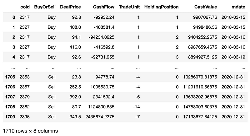
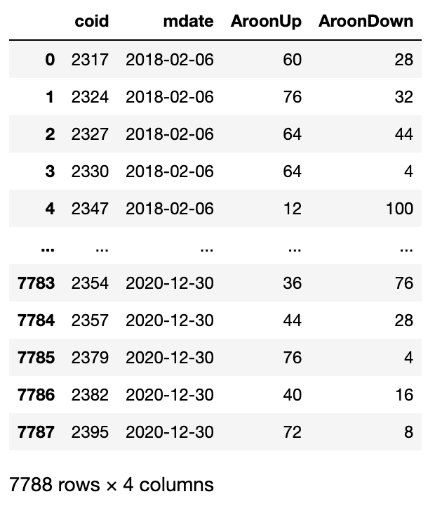
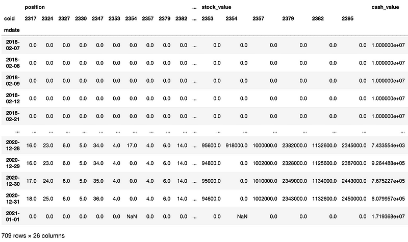
Today’s demo will be via the portfolio’s moving Alpha and Beta to assess the portfolio’s performance. To materialize it, first, we need to calculate the daily returns of the portfolio and market and then, respectively, store them in the new columns of the Portfolio Value Sheet.
value["total_value"] = value.apply(lambda x : x.sum(), axis = 1)
value["daily_return"] = value["total_value"].pct_change(periods=1)
value["market_return"] = list(stock[stock.coid == "Y9997"]["close_d"].pct_change(periods = 1)[25:])
value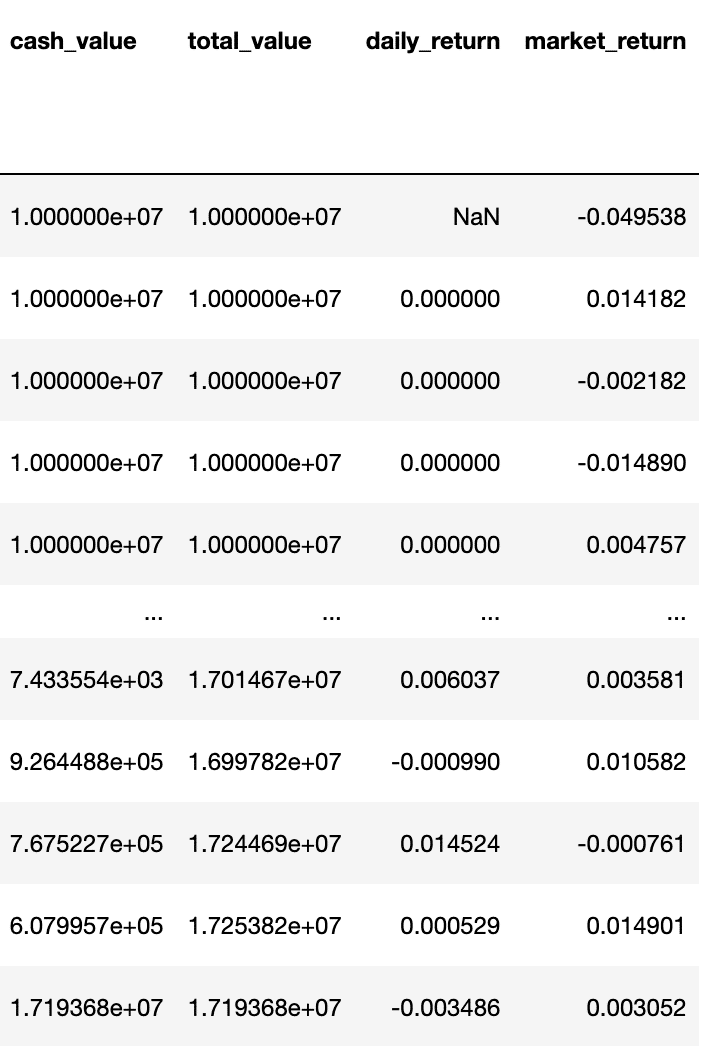
Next step, we will use “daily_return” and “market_return” as input variables to fit the Linear Regression model to get Alpha and Beta.
X = np.array(value["daily_return"].iloc[1:]).reshape(-1, 1)
y = np.array(value["market_return"].iloc[1:])
regressor = LinearRegression()
regressor.fit(X, y)
w_0 = regressor.intercept_
w_1 = regressor.coef_

print('alpha : ', w_0)
print('beta : ', w_1)
Let’s set our window as 60 days, calculate moving Alpha and Beta, and visualize the result.
window = 60
alpha = []
beta = []
mdate = []
for i in range(len(value) - window - 1):
    X = np.array(value["daily_return"].iloc[i+1 : i+1+window]).reshape(-1, 1)
    y = np.array(value["market_return"].iloc[i+1 : i+1+window])
    regressor = LinearRegression()
    regressor.fit(X, y)
    w_0 = regressor.intercept_
    w_1 = regressor.coef_
    alpha.append(round(w_0, 5))
    beta.append(w_1)
    mdate.append(value.index[i+1+window])
fig, ax1 = plt.subplots(figsize=[16, 9], constrained_layout=True)
ax1.plot(mdate, alpha, label = "Alpha")
ax1_2 = ax1.twinx()
ax1_2.plot(mdate, beta, label = "Beta", color = "orange")

Alpha_lines, Alpha_labels = ax1.get_legend_handles_labels()
Beta_lines, Beta_labels = ax1_2.get_legend_handles_labels()
ax1.legend(Alpha_lines + Beta_lines,
           Alpha_labels + Beta_labels, loc='upper right')

ax1.set_xlabel('mdate')
ax1.set_ylabel('Alpha')
ax1_2.set_ylabel('Beta')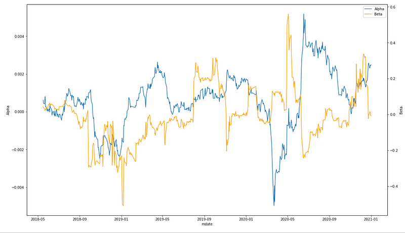
For the more profound analysis, we draw two line charts to compare the difference between each target’s and market trends and the variation of Aroon indicators during the backtesting period.
def make_plot(stock_df, aroon_dict, record_df, coid):
    # stock["mdate"] = stock["mdate"].apply(lambda x:x.strftime('%Y-%m-%d'))
    mdate = stock[stock.coid == "Y9997"].mdate

    benchmark = stock[stock.coid == "Y9997"].close_d

    AroonUp = aroon[aroon.coid == coid].AroonUp
    AroonDown = aroon[aroon.coid == coid].AroonDown
    aroon_date = aroon[aroon.coid == coid].mdate

    fig, axes = plt.subplots(2,1, figsize=[16, 9], constrained_layout=True)

    ax1 = axes[0]
    stock[stock.coid == "Y9997"].set_index("mdate").close_d.plot(ax = ax1, label = "market return")
    ax1_2 = ax1.twinx()
    stock[stock.coid == coid].set_index("mdate").close_d.plot(ax = ax1_2, label=f'{coid}_close', color = "lime")
    stock[stock.coid == coid].set_index("mdate").open_d.plot(ax = ax1_2, label=f'{coid}_open', color = "deeppink", alpha = 0.5)
    ax1_2.scatter(df[df.coid == coid].mdate, df[df.coid == coid].DealPrice, label = "BuyOrSell", color = ["orange" if i == "Buy" else "purple" for i in df[df.coid == coid].BuyOrSell])

    benchmark_lines, benchmark_labels = ax1.get_legend_handles_labels()
    target_lines, target_labels = ax1_2.get_legend_handles_labels()

    ax1.legend(benchmark_lines + target_lines,
               benchmark_labels + target_labels, loc='upper right')
    ax1.set_xlabel('mdate')
    ax1.set_ylabel('index')
    ax1_2.set_ylabel(f'price')
    ax1.set_title(f"{coid}_Aroon")

    ax2 = axes[1]
    aroon[aroon.coid == coid].set_index("mdate").AroonUp.plot(ax = ax2, label = "AroonUp", color = "red")
    ax2_2 = ax2.twinx()
    aroon[aroon.coid == coid].set_index("mdate").AroonDown.plot(ax = ax2_2, label = "AroonDown", color = "green")

    up_lines, up_labels = ax2.get_legend_handles_labels()
    down_lines, down_labels = ax2_2.get_legend_handles_labels()

    ax2.legend(down_lines + down_lines,
               up_labels + down_labels, loc='upper right')
    ax2.set_xlabel('mdate')
    ax2.set_ylabel('Aroon_indicator')

    fig.tight_layout()

    plt.show()
We can easily generate each target’s charts by using for loop.
Please note that because the last item of stock.coid.unique() is the market’s id “Y9997,” our range of for loop would not contain the last item.
for coid in stock.coid.unique()[:-1]:
    make_plot(stock, aroon, value, coid)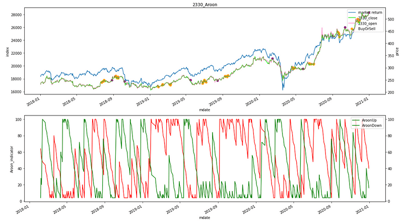
In the first chart, the blue line is the market index, the green line is the target’s closing price, and the pink line is the opening price. And the yellow points are the buying points, and the purple points are the selling points.
In the second chart, the red line is the Aroon-up indicator, and the green line is the Aroon-down indicator.
While calculating the portfolio performance and market performance, we find out that the former’s return transcends the latter’s return about 17 percent.
print(f'大盤總績效:{stock[stock.coid == "Y9997"].close_d.iloc[-1]/stock[stock.coid == "Y9997"].close_d.iloc[0] -1}')
print(f'投資組合總績效:{value["total_value"].iloc[-1]/value["total_value"].iloc[0] -1}')
Through the chart of Moving Alpha & Beta, we can conclude that our strategy is arguably conservative. Its fluctuation of Alpha and Beta are both mild; On the other hand, each target’s own buying and selling points are clearly seen by each target’s first chart. So we can analyze which target in the portfolio is the backbone of profit. Furthermore, investors can freely adjust or customize the Aroon indicators trading strategy in accordance with their own stock-picking strategy to fulfill a one-stop system from stock picking and automated trading to performance assessing.
Last but not least, please note that “Stocks this article mentions are just for the discussion, please do not consider it to be any recommendations or suggestions for investment or products.” Hence, if you are interested in issues like Creating Trading Strategy , Performance Backtesting , Evidence-based research , welcome to purchase the plans offered in TEJ E Shop and use the well-complete database to create your own optimal trading strategy.