Programming CRR model for calculating options theoretical price.

Table of Contents
In our previous article — 【Quant】Black Scholes model and Greeks, we introduce how to program the Black Scholes model. However, Black Scholes has its disadvantages and can not calculate the theoretical price for American options. Therefore, three years after the appearance of Black Scholes, John Cox, Stephen Ross, and Mark Rubinstein invented a relatively easy and more general options pricing model — the CRR model.
The CRR model uses the binomial theorem to discretize the future, assuming that there are only two possibilities for each time point — an up or a down movement — and that the magnitude of the movements is fixed. In this way, the future price of the underlying asset can be plotted as a binary tree model as time progresses. Then, calculate the intrinsic value of the option under each node, and take the present value of each node to derive the option’s theoretical value by working backward.
Windows 11 and Jupyter Notebook are used as editor
# Load required package
import math
import tejapi
import pandas as pd
import numpy as np
import matplotlib.pyplot as plt
from scipy.stats import norm
plt.style.use('ggplot')

# log in TEJ API
api_key = 'YOUR_KEY'
tejapi.ApiConfig.api_key = api_key
tejapi.ApiConfig.ignoretz = TrueStock trading database: Unadjusted daily stock price, database code is (TWN/APRCD).
Derivatives database: Options daily transaction information, database code is (TWN/AOPTION).
Using the unadjusted close prices of the Taiwan Weighted Index (Y9999), from January 1, 2021, to April 19, 2023. And loading the Taiwan Weighted Index Call, Put Option (TXO202304C15500, TXO202304P15500), which are European options, with a start trading date of January 1 and an expiration date of April 19, and a strike price of 15500.
# set time zone
gte, lte = '2021-03-16', '2023-04-20'

# Get stock price
stocks = tejapi.get('TWN/APRCD',
                   paginate = True,
                   coid = 'Y9999',
                   mdate = {'gte':gte, 'lte':lte},
                   opts = {
                       'columns':[ 'mdate','close_d']
                   }
                  )

# Get options price
puts = tejapi.get( # puts price
    'TWN/AOPTION',
    paginate = True,
    coid = 'TXO202304P15500',
    mdate = {'gte':gte, 'lte':lte},
    opts = {
        'columns':['mdate', 'coid','settle', 'kk', 'theoremp', 'acls', 'ex_price', 'td1y', 'avolt', 'rtime']
    }
)
calls = tejapi.get( # calls price
    'TWN/AOPTION',
    paginate = True,
    coid = 'TXO202304C15500',
    mdate = {'gte':gte, 'lte':lte},
    opts = {
        'columns':['mdate', 'coid','settle', 'kk', 'theoremp', 'acls', 'ex_price', 'td1y', 'avolt', 'rtime']
    }
)

# set index
stocks = stocks.set_index('mdate')
puts = puts.set_index('mdate')
calls = calls.set_index('mdate')Calculating daily return and moving volatility, set 252 days as the window.
# Calculate stock return and moving volatility
stocks['daily return'] = np.log(stocks['close_d']) - np.log(stocks['close_d'].shift(1))
stocks['moving volatility'] = stocks['daily return'].rolling(252).std()As previously mentioned, the CRR model is a more intuitive and flexible options pricing model than Black Scholes. Although it does not have a closed-form solution like Black-Scholes and may be more time-consuming to calculate due to its binary tree structure, the CRR model has advantages over Black-Scholes in pricing options with time-varying characteristics, such as American options and exotic options.
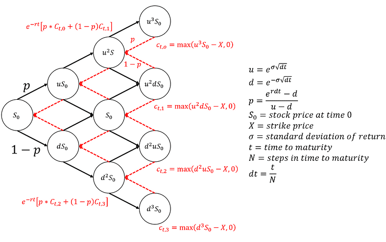
The basic formula of the CRR model is to calculate the present value of each node in the binary tree. We can use the following formula to calculate the magnitude and probability of stock price movements in the next period, denoted as u, d, and p, in the diagram below. Then, we can calculate the stock prices going up and down in the following period and form a tree structure as time passes. The black lines and mathematical formulas in the diagram represent the changes in stock prices, while the red lines and mathematical formulas represent the call option’s value. We can see that we first calculate the future changes in stock prices (e.g., uS0, dS0), then subtract the strike price from the stock price to obtain the intrinsic value of the call option (e.g., Ct,1, Ct,2), and finally, step by step, we can calculate the present value of the call option and obtain the theoretical price of the option today.
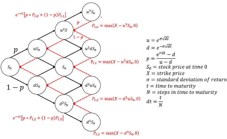
For put options, we just need to change the method of calculating the intrinsic value by subtracting the stock price from the strike price (e.g., Pt,0, Pt,1). The rest of the calculation process is the same as for call options in the CRR model.
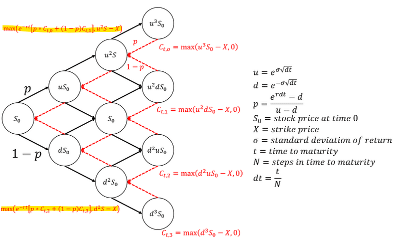
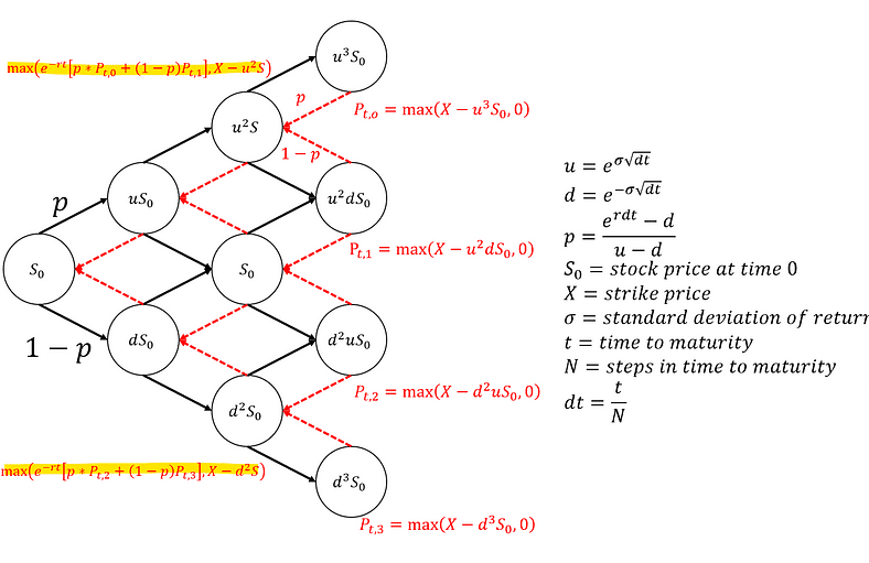
Compared to Black Scholes, the CRR model can price American-style options. The so-called American options allow the option holder to exercise the option before the expiration date, while the regular options are called European options. For the holder, as long as the current intrinsic value is greater than the present value obtained by backward induction, there is an incentive to exercise the option. Therefore, the option price at each node will be the maximum value between the present value obtained by backward induction and the intrinsic value, as shown in the highlighted part of the diagram.
After understanding how to calculate options prices using the CRR model, we will move on to the programming part.
class crr_model:

    # init fuction
    def __init__(self, s, x, r, t, sigma, N, sigma_daily = True):

        t /= 252
        dt = t/N
        if sigma_daily:
            sigma *= np.sqrt(252)
        u = np.exp(sigma * math.sqrt(dt))
        d = 1/u
        p = (np.exp(r*dt)-d) / (u-d)

        self.s = s
        self.x = x
        self.r = r
        self.t = t
        self.N = N
        self.dt = dt
        self.u = u
        self.d = d
        self.p = p
        self.sigma = sigma

    # european call price
    def eu_call_price(self):

        lattice = np.zeros((self.N+1, self.N+1))
        for j in range(self.N+1):
            lattice[self.N, j] = max(0, self.s*(self.u**j)*(self.d**(self.N-j)) - self.x)
        for i in range(self.N-1, -1, -1):
            for j in range(i+1):
                lattice[i, j] = np.exp(-self.r*self.dt)*(self.p*lattice[i+1,j+1] + (1-self.p) * lattice[i+1, j])

        return lattice[0,0], lattice

    # european put price
    def eu_put_price(self):

        lattice = np.zeros((self.N+1, self.N+1))
        for j in range(self.N+1):
            lattice[self.N, j] = max(0, self.x - self.s*(self.u**j)*(self.d**(self.N-j)))
        for i in range(self.N-1, -1, -1):
            for j in range(i+1):
                lattice[i, j] = np.exp(-self.r*self.dt)*(self.p*lattice[i+1,j+1] + (1-self.p) * lattice[i+1, j])

        return lattice[0,0], lattice

    # american call price
    def am_call_price(self):

        lattice = np.zeros((self.N+1, self.N+1))
        for j in range(self.N+1):
            lattice[self.N, j] = max(0, self.s*(self.u**j)*(self.d**(self.N-j)) - self.x)
        for i in range(self.N-1, -1, -1):
            for j in range(i+1):
                lattice[i, j] = max(np.exp(-self.r*self.dt)*(self.p*lattice[i+1,j+1] + (1-self.p) * lattice[i+1, j]),
                                   self.s*(self.u**j)*(self.d**(i-j)) - self.x )

        return lattice[0,0], lattice

    # american put price
    def am_put_price(self):

        lattice = np.zeros((self.N+1, self.N+1))
        for j in range(self.N+1):
            lattice[self.N, j] = max(0, self.x - self.s*(self.u**j)*(self.d**(self.N-j)))
        for i in range(self.N-1, -1, -1):
            for j in range(i+1):
                lattice[i, j] = max(
                    np.exp(-self.r*self.dt)*(self.p*lattice[i+1,j+1] + (1-self.p) * lattice[i+1, j]),
                    self.x - self.s*(self.u**j)*(self.d**(i-j))
                                   )

        return lattice[0,0], lattice
To replicate the tree structure, we use a nested array of numpy to form an (N+1) x (N+1) matrix, where the top-left element is the option’s theoretical price. The blue line in the lower left corner is the aforementioned tree diagram.
s = 100 # set stock price at time 0
x = 95 # set strike price
r = 0 # set risk-free rate = 0%
t = 252 # set time to maturity at 252 days
sigma = 0.3 # set annualized volatility at 0.3
N = 4 # set steps at 4

crr = crr_model(s, x, r, t, sigma, N, sigma_daily = False)
call, call_lat = crr.eu_call_price()
call_lat
Keen-eyed readers may have noticed the existence of the variable N, which can be viewed as the number of times the expiration period is divided. For example, if the time to maturity is 252 days and N is set at 251, it means that the future stock price is calculated once a day, and the tree diagram will have 252 layers. That is, the number of layers (N+1) of our tree is determined by N. The question is, what is the optimal value for N to achieve better pricing results? In fact, there is no specific N value, but we can observe that as we increase the number of N, that is, divide time into smaller segments, the calculated option price will approach a constant value. Therefore, if the computer power permits, a higher N value would be better.
# plot the convergency pattern of crr model

calls_ = []
for n in range(1, 100):

    s = 100
    x = 100
    r = 0.011
    t = 52
    sigma = 0.3

    crr = crr_model(s, x, r, t, sigma, n, sigma_daily = False)
    call, call_lat = crr.eu_call_price()
    calls_.append(call)

plt.plot(range(1, 100), calls_, color = 'red')
plt.xlabel('Numbers of N')
plt.ylabel('Theoretical call price')
plt.title('Options price convergency')
plt.savefig('Options price convergency')
plt.show()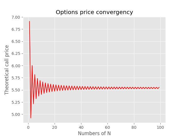
Finally, let’s compare the theoretical prices obtained through the CRR model with the Black Scholes price calculated by TEJ and the actual market price.
We use a TAIEX put option with a strike price of 15500, from January 1, 2023, to April 19, 2023. The risk-free rate is set at the yield of the Taiwan 5-year bond (0.011), and Sigma uses the standard deviation of TAIEX returns over a 252-day window. N is set to 1000. The results obtained are shown below, and it can be seen that the CRR price is closer to the actual market price than the Black Scholes price calculated by TEJ.
s = stocks.loc['2023-01-31']['close_d'] # get the stock price at the first dat of options trading
x = 15500 # strike price
r = 0.011 # use 5-year Taiwan government bond ytm
t = 51 # time to maturity
sigma = stocks.loc['2023-01-31']['moving volatility'] # get the return volatility at the first day od options trading
N = 100 # divided time 2 maturity into 10 parts

crr = crr_model(s, x, r, t, sigma, N, sigma_daily = True)
call, call_lat = crr.eu_call_price() # european call price
put, put_lat = crr.eu_put_price() # european put price
call_a, call_lat_a = crr.am_call_price() # american call price
put_a, put_lat_a = crr.am_put_price() # american put price

print('CRR theoretical price: ', put)
print('TEJ Black Scholes price: ', puts.loc['2023-01-31']['theoremp'])
print('Real price: ', puts.loc['2023-01-31']['settle'])
The CRR model, as a newcomer, offers more flexibility than the Black-Scholes model. In the wave of derivative products that followed, many unique options can be priced using the CRR model or its extension models. Its simple mathematical calculation method and theoretical basis make it a good choice for many novice option investors. In this article, we have completed the programming of the CRR model for pricing European and American options. We will provide more knowledge related to options or derivative products in the future. Please continue to follow us, and readers and investors are also welcome to purchase TEJ E Shop to build their option pricing programs. Please note that the pricing formulas and options products mentioned above are for demonstration purposes only and do not represent any investment or target recommendations.