
Photo by Isaac Smith on Unsplash
Table of Contents
First of all, we need to declare the Time Series concept. It is a kind of data structure showing the development of historical data by the order of time. As for Time Series Model, it is applied to analyze time series data. Further, by this model, we manage to find high-likelihood trend and make forecasting.
Models we will implement are as follow:
Autoregressive Integrated Moving Average model, ARIMA
ARIMA is a fundamental time series model. Its parameters are Autoregression(AR), Differencing and Moving Average(MA).
General Autoregressive Conditional Heteroskedasticity model, GARCH
GARCH is used to analyze time series error. It is especially useful with application to measure volatility in investment domain. We will implement GARCH model to test residual from ARIMA so as to modify the error term. Parameters of GARCH is similar to that of ARIMA, but GARCH mainly focuses on error and variance. As for the numbers of (p,q), which is the amount we take from lagged data to fit GARCH, we will determine by ACF/PACF with the consideration of GARCH’s characteristics.
Process Outline:
MacOS & Jupyter Notebook
# 基本功能
import numpy as np
import pandas as pd# 繪圖
import matplotlib.pyplot as plt
%matplotlib inline
import seaborn as sns
sns.set()# TEJ API
import tejapi
tejapi.ApiConfig.api_key = 'Your Key'
tejapi.ApiConfig.ignoretz = True
0050.TW is target index in this article.
data_price = tejapi.get('TWN/EWPRCD', # 公司交易資料-收盤價
                  coid= '0050', # 台灣50
                  mdate={'gte': '2003-01-01', 'lte':'2021-12-24'},
                  opts={'columns': ['coid', 'mdate', 'close_d', ]},
                  chinese_column_name=True,
                  paginate=True)
data_price = data_price.set_index('日期')# 導入中文
plt.rcParams['font.sans-serif'] = ['Arial Unicode MS']# 繪製0050價格走勢圖
fig, ax = plt.subplots(figsize = (10, 5))
plt.plot(data_price['收盤價'], label = '0050-price')
plt.title('0050收盤價')
plt.legend()
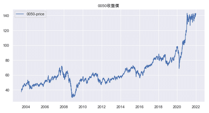
Based on above chart, it is clear that there exists a trend with time elapse. This situation is caused by that price data is non-stationary. Therefore, we conduct Augmented Dickey-Fuller(ADF) Test to check whether unit root exists in the series or not. If unit root truly exists, we would “difference” raw data to convert non-stationary to stationary. We will check this by P-value.
# 從statsmodels數據包導入ADF套件
from statsmodels.tsa.stattools import adfuller# 從產出的ADF報表擷取P-value項目
price_p_value = adfuller(data_price['收盤價'])[1]# 設定判別式以及0.05的P-value標準
if price_p_value > 0.05:
    print('Nonstationary')
else:
    print('Stationary')
H0:Data is Non-stationary
H1:Data is Stationary
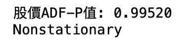
According to the result of ADF test, it is assured that price data is non-stationary. Hence, we cannot take price to fit following models.
Reason to declare the importance of being stationary or not is as follow:
If data is non-stationary, its trend would be random walk. As a result, it is just a coincidence that data fits model well. It is non-sense to prove how-well a model performs. After all, model cannot interpret a random walk.
As know that price is not eligible for fitting model, we import “Return ”(Graph and ADF process is available in the Source Code)
data_ret = tejapi.get('TWN/EWPRCD2', # 公司交易資料-報酬率
                  coid= '0050', # 台灣50
                  mdate={'gte': '2003-01-01', 'lte':'2021-12-24'},
                  opts={'col     umns': ['coid', 'mdate', 'roia', ]},
                  chinese_column_name=True,
                  paginate=True)
data_ret = data_ret.set_index('日期')
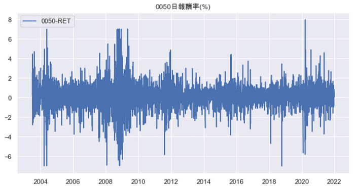
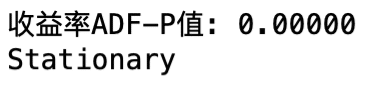
According to the result of ADF test, it is assured that return data is stationary. Hence, we can take price to fit following models.
train_date = data.index.get_level_values('日期') <= '2020-12-31'
train_data = data[train_date]
test_data = data[~train_date]
- train_data:Serve as the term to construct model
- test_data: Serve as the term to compare with the post-modelling prediction
This article would only focus on data pre-processing and modelling, so we would apply test_data only in following article.
We apply pmdarima to find best-fitted parameter set.
import pmdarima as pmdpmd_mdl = pmd.auto_arima(train_data['日報酬率(%)'], stationary = True)
pmd_mdl.summary()
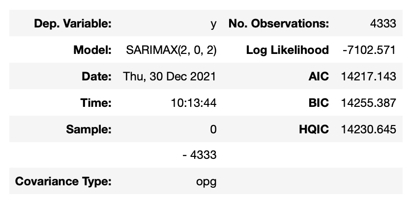
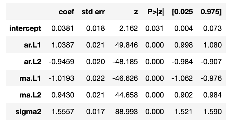
According to above table, we would know that the best-fitted parameter set is (2, 0, 2). To boot, it is clear that every P-value is smaller than the strictest level, 0.01, so the significance of every coefficient is certain.
Note:If you notice that the name of model is SARIMAX, instead of ARIMA, it is nothing to worry about. SARIMAX is the default set of pmdarima, but the process remains ARIMA. We import statsmodel package to check this result.
from statsmodels.tsa.arima.model import ARIMAmodel = ARIMA(train_data['日報酬率(%)'], order = (2, 0, 2))
stats_mdl = model.fit()
print(stats_mdl.summary())
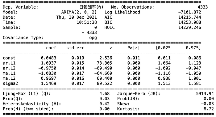
Observing the ARIMA report by statsmodels, we know the difference of fitting level(AIC & BIC) between pmdarima and statsmodels is tiny. As for the coefficient estimation table, the significance level is identical as well, though the coefficient and standard error terms differs a little.
Residual diagnosis
stats_mdl.plot_diagnostics(figsize = (15, 10))
plt.show()
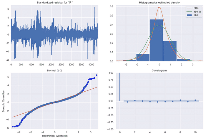
There is no apparent trend of residual by observing left-top chart. However, the histogram(right-top) and Normal Q-Q plot(left-bottom) make us conclude that the normality of model residual is not sufficient, which indicates that ARIMA’s residual still contains some explanatory variable. We would conduct white noise test to verify it.
White Noise Test
By Ljung-Box Test, we would know whether ARIMA’s residual is random or not. If the result shows that residual is white noise(random), we could conclude that ARIMA is fitted well. However, if residual is not white noise, we would further implement GARCH to interpret the explanatory variance inside error term.
from statsmodels.stats.diagnostic import acorr_ljungboxwhite_noise = acorr_ljungbox(pmd_residual, lags = [10], return_df=True)
H0:Error term is white noise
H1:Error term is not white noise
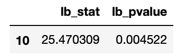
Test result make us know the error term is not white noise(P-value < 0.05). Therefore, we would conduct GARCH to fit ARIMA’s residual.
ARCH Effect Test
In spite of proof of that ARIMA’s residual is not random, we cannot prove that term exists heteroskedasticity. We would conduct ARCH Effect Test to confirm that.
from statsmodels.stats.diagnostic import het_archLM_pvalue = het_arch(arima_resid, ddof = 4)[1]
print('LM-test-Pvalue:', '{:.5f}'.format(LM_pvalue))
H0: ARCH Effect not exists
H1:ARCH Effect exists

By P-value of the test, we would reject H0. Namely, we can apply GARCH to fit ARIMA’s residual.
透過觀察殘差ACF/PACF圖,了解殘差平方項目的滯後情形,並將觀察到的結果帶入GARCH模型中,決定GARCH模型的參數組合,檢定波動度。
fig, ax = plt.subplots(1, 2, figsize = (18,5))pmd_residual = pmd_mdl.arima_res_.resid
sgt.plot_acf(pmd_residual**2, zero = False, lags = 40, ax=ax[0])
sgt.plot_pacf(pmd_residual**2, zero = False, lags = 40, ax=ax[1])plt.show()
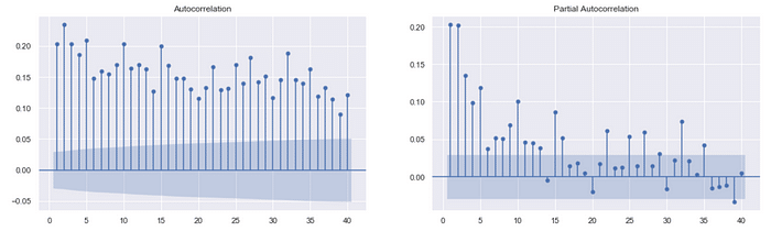
Above chart makes us know that squared-residual’s autoregression is significant. Synthesizing PACF(right) and GARCH’s mathematics structure, we assume that GARCH’s parameter set (p,q) are (1,1), (2,1), (1,2) and (2,2). After compare model’s goodness of fit and significance of those sets, we determine which set to use. In case of the redundant content, we only display the best-fitted set, (1,1).
Note:GARCH’s mathematics structure contains all the historical data and the weight becomes lower as the time farer.
from arch import arch_modelmdl_garch = arch_model(pmd_residual, vol = 'GARCH', p = 1, q = 1)
res_fit = mdl_garch.fit()
res_fit.summary()
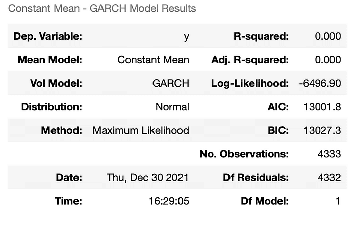
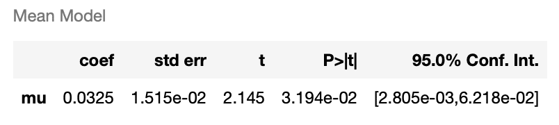
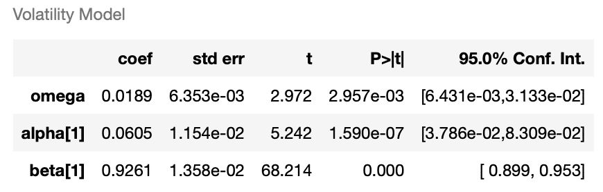
According to above tables, we understand that every coefficient is significant. The following is diagnosis of GARCH model.
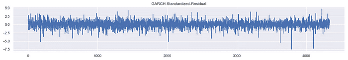
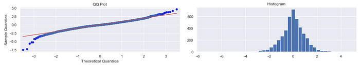
Observing above chart, we can conclude that there is no trend for GARCH residual. On top of that, based on residual histogram and Normal Q-Q plot show the normality. Again, we apply white noise test to further verify that residual is random.
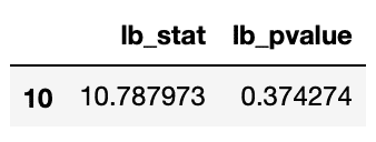
Test result make us know the error term is white noise(P-value > 0.05). Therefore, no explanatory variable can be taken. The residual is random.
So far, we have gone through the whole process of modeling. Firstly, verify non-stationary and stationary data. Secondly, fit ARIMA model with return data. Lastly, fit GARCH model with residual term. You may notice the process of Statistics test is very strict. This article, however, in order to make readers acquainted with whole process quickly, spare mathematics theorems behind models and tests.
The above implementation of time series model is what we expect readers to understand. Following article would discuss how to apply the models to forecasting. Last but not least, credit to database of TEJ, we can easily conduct tests and models. As a result, welcome to purchase the plan offered in TEJ E-Shop to find the data you need.
