
Through the previous 2 articles of “Data Analysis” , we have shared with you how to use Numpy and Pandas to start the first step of data analysis and the importance of using the adjusted stock price if you want to calculate the return. Therefore, this time we are going to use those tools to do the “dollar-cost averaging method” backtesting and let you see the power of compound interests!
Table of Contents
Backtesting means that after having a strategy, you can invest by selecting the underlying asset, buying/selling signals, or using portfolio methods and combine with the historical data to test the strategy in order to understand how it performed in the past. Then, use this result as one of the important parameters for future investment decisions. For example:Assumption:As long as the company’s ROE exceeds 15%, then we buy it’s stock, rebalance once a year, and sell when its ROE falls below 15%.
This kind of thought can actually create so-called backtesting because you already have those parameters we have mentioned above. However, there are still some ⚠points that need to be noted⚠ when we do backtesting, which will be shared with you later.
In Taiwan, the DCA method is getting more popular and popular among retail investors. But what is the DCA method? Is that good? When this kind of thought appears, it’s time for backtesting!
Noun Definition:
1. 0050.TW(ETF): Tracking Taiwan 50 Index, and the constituent stocks include the top 50 market value listed companies in Taiwan.
2. Dollar-Cost Averaging(DCA) method: An investment strategy of buying a fixed amount of money with every certain period.
Our strategy:
At the beginning of each month, we will invest NT$10,000 for total 5 years. During this period, we won’t withdraw our money and the transaction costs will be ignored.
import pandas as pd
import numpy as np
import matplotlib.pyplot as plt
import matplotlib.ticker as ticker
import matplotlib.transforms as transformsimport datetimeimport tejapi
tejapi.ApiConfig.api_key = “your key”
2. Data collection from TEJ APITW0050 = tejapi.get(
‘TWN/EWPRCD’,
coid = ‘0050’,
mdate={‘gte’:’2016-01-01′, ‘lte’:’2020-12-31′},
opts={‘columns’: [‘mdate’,’close_adj’]},
paginate=True
)
TW0050[‘mdate’] = TW0050.loc[:,’mdate’].astype(‘datetime64[ns]’)
TW0050 = TW0050.set_index(‘mdate’)##change the frequency of the data
TW0050_monthly = TW0050.resample(‘MS’).first()##add the last day of our historical data
TW0050_monthly = TW0050_monthly.append(TW0050.iloc[-1])
TW0050_monthly
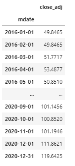
As we can see from the codes above, after getting the data from TEJ API, we first set the date data to index, and then use the pandas.resample() function to convert the daily data to monthly data. Last, because we want to know the return rate on the last day of this period, we add the data point of 2020–12–31 to our dataframe.
3. Calculate relevant information for each period##Shares to buy in each month(chop off)
TW0050_monthly[‘每月購買股數’]=
np.floor(10000 / TW0050_monthly[‘close_adj’])TW0050_monthly[‘每月購買股數’][-1] = 0##Cumulative Shares
TW0050_monthly[‘累積股數’] = TW0050_monthly[‘每月購買股數’].cumsum()##Cumulative Shares Value
TW0050_monthly[‘累積價值(月)’] =
round(TW0050_monthly[‘累積股數’] * TW0050_monthly[‘close_adj’],2)##Original Asset Value
TW0050_monthly[‘原始價值(月)’] =
[10000*i for i in range(len(TW0050_monthly.index))]TW0050_monthly[‘原始價值(月)’] =
TW0050_monthly[‘原始價值(月)’].shift(-1)TW0050_monthly[‘原始價值(月)’][-1] = TW0050_monthly[‘原始價值(月)’][-2]##Cumulative Return
TW0050_monthly[‘累積報酬(月)’] =
round((TW0050_monthly[‘累積價值(月)’]-TW0050_monthly[‘原始價值(月)’])/TW0050_monthly[‘原始價值(月)’], 6) +1
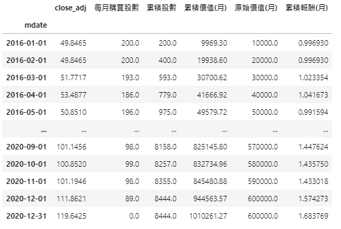
From those formulas above we could know that we just simply calculate the value of our total shares each month. Then, we compare with the original asset at the same time period to get this conclusion:
We start to buy the 0050.TW ETF equal to the value of NT$10,000 since 2016 Jan every month. After 5 years, the total number of shares are 8,444 shares, the cumulative value is around 1,010,261, and the cumulative return is 68%.
4. Data Visualization
Let’s use a graph to look at the changes in assets.plt.figure(figsize = (10, 6))
plt.plot(TW0050_monthly[‘累積價值(月)’], lw=1.5, label = ‘0050’)
plt.plot(TW0050_monthly[‘原始價值(月)’], lw=1.5, label = ‘Original Asset’)
plt.xlabel(‘Time(Year)’)
plt.ylabel(‘Value’)
plt.legend(loc = 0)
plt.grid()
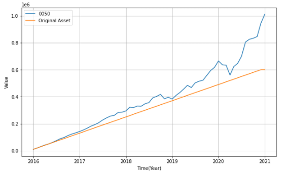
It could be found that most of the growth occurred last year. The increase is relatively slow if we exclude 2020. Therefore, this investing method takes time to see the increase of our assets.💪💪
Then what if we want to know the monthly return?##Monthly return
ret =
np.log(TW0050_monthly[‘累積報酬(月)’]/TW0050_monthly[‘累積報酬(月)’].shift(1))fig, ax = plt.subplots()
ret.plot(kind=”bar”, figsize=(12,6), stacked=True, ax=ax)##Build an empty array with the length of total data
ticklabels = [”]*len(TW0050_monthly.index)##Show the month and the date every 6 months
ticklabels[::6] =
[item.strftime(‘%b %d’) for item in TW0050_monthly.index[::6]]##Show the year every 12 months
ticklabels[::12] =
[item.strftime(‘%b %d\n%Y’) for item in TW0050_monthly.index[::12]]ax.xaxis.set_major_formatter(ticker.FixedFormatter(ticklabels))
plt.gcf().autofmt_xdate()##Add the horizontal line of average monthly return
ax.axhline(ret.mean(), c=’r’)plt.xlabel(‘Month’)
plt.ylabel(‘Return’)
plt.title(‘0050 Monthly return’)plt.show()
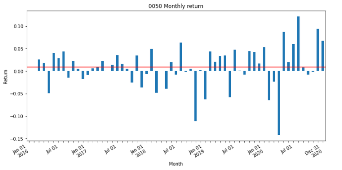
From the graph, we could know that most of the monthly returns are within a certain range except for 2020.
5. Performance/Statistic Indicators
Finally, we may be able to analyze this strategy through some performance indicators.##CAGR
cagr = (TW0050_monthly[‘累積報酬(月)’][-1]) ** (1/5) -1##Annually Standard Deviation
std = ret.std()*np.sqrt(12)##Sharpe Ratio(Assume that Rf is 1%)
shapre_ratio = (cagr-0.01)/std##MDD
roll_max = TW0050_monthly[‘累積價值(月)’].cummax()
monthly_dd =TW0050_monthly[‘累積價值(月)’]/roll_Max – 1.0
max_dd = monthly_dd.cummin()##Table
pd.DataFrame(columns=[‘0050’],
index=[‘年化報酬率(%)’, ‘年化標準差(%)’, ‘夏普比率’, ‘期間最大回撤(%)’],
data = np.round(np.array([100*cagr, 100*std, sharpe_ratio, 100*max_dd[-1]]),2))
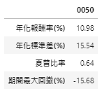
According to our investment method, we could know that using this DCA method can get an annualized rate of return around 11%, which is quite a high number because the deposit rate of banks is around only 1%. Through the effect of compound interest, the original asset will increase about 1.6 times the original in 5 years, and the volatility and the Sharpe ratio perform not bad as well.
But in terms of disadvantages, this method will still be affected by the volatility caused by systematic risks such as COVID-19 due to the properties of this ETF. Moreover, the time when we want to sell the stocks and make a profit depends on the investors’ decision.
DCA method is a easy and convenient strategy for many people who are new to investment. However, People who use this method must have a strong discipline such as entering the market every month no matter what happens at that time and keeping holding that assets for many years. Therefore, it is not suitable for people who don’t have enough money to do this operation.
In this article, we use backtesting to understand how our strategy performed in the past. But the past does not mean the future. It just allows investors to prove their ideas or strategies which are workable in the past so as to make a reference for the future.
To make successful backtesting, we still need to pay attention to things such as the data quality, the length of data, whether there are bugs in your program, whether too many transaction costs are ignored, etc. As long as there is a mistake in these problems, it will cause the distortion of the backtesting and lose money!! As a result, you have to pay attention to our backtesting result again️️️️️️️️️️️ every time