
Table of Contents
In 1997, Robert Merton and Myron Scholes won the Nobel Prize in Economics for their Black-Scholes options pricing formula, beating out many other contenders. The Black-Scholes model is still a widely-used option pricing model in the financial industry and by investors due to its excellent mathematical properties, simplicity, and ease of use. Today, we will focus on programming this model and Greeks derived from Black Scholes model.
Windows 11 and Jupyter Notebook is used as editor
# 載入所需套件
import math
import tejapi
import pandas as pd
import numpy as np
import matplotlib.pyplot as plt
from scipy.stats import norm
plt.style.use('bmh')
plt.rcParams['font.sans-serif']=['Microsoft YaHei']

# 登入TEJ API
api_key = 'YOUR_KEY'
tejapi.ApiConfig.api_key = api_key
tejapi.ApiConfig.ignoretz = TrueStock trading database: Unadjusted daily stock price, database code is (TWN/APRCD).
Derivatives database: Options daily transaction information, database code is (TWN/AOPTION).
Before running simulations, however, practitioners must collect accurate and high-frequency market data to serve as input for these models. Whether you’re modeling volatility, interest rate changes, or stock price movements, reliable historical data is the foundation of any sound pricing strategy.
If you’re looking to apply option pricing techniques in practice, start with TEJ Market Data —a comprehensive solution for time-series stock prices, implied volatility, and benchmark interest rates that are essential for simulation-based pricing.
Using the unadjusted close prices of the Taiwan Weighted Index (Y9999), with a time period from March 16, 2021 to April 10, 2023. And loading the Taiwan Weighted Index Call Option (TXO202304C15500), which is a European call option, with a start trading date of March 16 and an expiration date of April 19, and a strike price of 15500.
gte, lte = '2021-03-16', '2023-04-10'
# 標的物價格
stocks = tejapi.get('TWN/APRCD',
                   paginate = True,
                   coid = 'Y9999',
                   mdate = {'gte':gte, 'lte':lte},
                   chinese_column_name = True,
                   opts = {
                       'columns':[ 'mdate','close_d']
                   }
                  )
# 選擇權價格
options = tejapi.get(
    'TWN/AOPTION',
    paginate = True,
    coid = 'TXO202304C15500',
    mdate = {'gte':gte, 'lte':lte},
    chinese_column_name = True,
    opts = {
        'columns':['mdate', 'coid','settle', 'kk', 'theoremp', 'acls', 'ex_price', 'td1y', 'avolt', 'rtime']
    }
)
# 重設日期為index
stocks = stocks.set_index('年月日')
options = options.set_index('日期')Calculating daily return and moving return volatility with a window of 252 days.
stocks['日報酬'] = np.log(stocks['收盤價(元)']) - np.log(stocks['收盤價(元)'].shift(1))
stocks['移動報酬波動度'] = stocks['日報酬'].rolling(252).std()
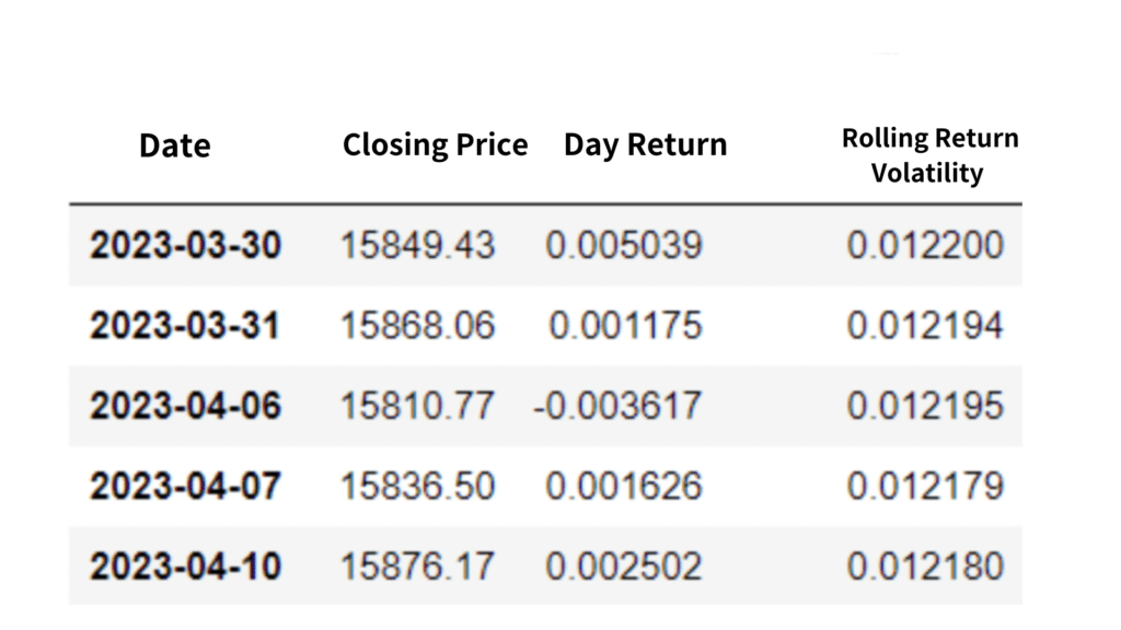
The resultant dataframe after processing is shown below:
First, we can take a look at the formula before programming.
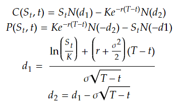
● C(St, t), P(St, t) : call, put price at day t.
● St, K : price of underlying asset and strike price at day t.
● T, t : Maturity date and day t.
● sigma : historical moving return volatility, in here, we take a window of 252 days.
● r : risk-free rate.
● N() : cumulative density function of standard normal distribution.
By observing above formula, we can see that there are 5 factors affecting options theoretical price: underlying asset price, strike price, time to maturity(T-t), return volatility and risk-free rate. Apart from strike price, other four factors are time-varying. In order to study the relationships between these four factors and options price, Greeks are invented to quantify the relationships. They are delta, gamma, vega, theta and rho.
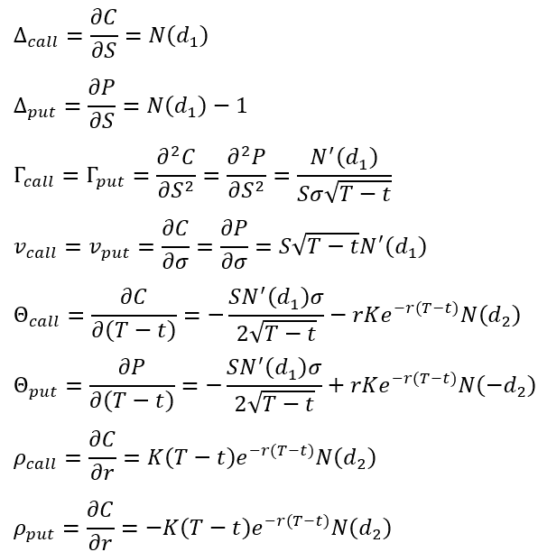
The concepts of Greeks are simple. They are just the partial derivatives of options price with respect to underlying asset price, volatility, time to maturity and risk-free rate. In particular, gamma is the second-order partial derivatives of options price with respect to underlying asset price. Thanks to the effort from those great ancient mathematicians, every single Greeks has an analytic solution, so we don`t have to deal with those nasty partial derivative function😆.
The below graph presents all Greeks analytic solutions. From top to bottom, there are delta of call, delta of put, gamma of call and put, vega of call and put, theta of call, theta of put, rho of call, rho of put.
Without further ado, let me just show you the code😎.
class BS_formula:
    def __init__(self, s0, k, r, sigma, T):
        self.s0 = s0 # 標的物價格
        self.k = k # 履約價格
        self.r = r # 無風險利率
        self.sigma = sigma # 歷史波動度
        self.T = T # 剩餘到期時間
        self.d1 = (np.log(s0/k)+(r+sigma**2/2)*T) / (sigma * np.sqrt(T))
        self.d2 = ((np.log(s0/k)+(r+sigma**2/2)*T) / (sigma * np.sqrt(T))) - sigma*np.sqrt(T)

    def BS_price(self): # 計算理論價格
        c = self.s0*norm.cdf(self.d1) - self.k*np.exp(-self.r*self.T)*norm.cdf(self.d2)
        p = self.k*np.exp(-self.r*self.T)*norm.cdf(-self.d2) - self.s0*norm.cdf(-self.d1)
        return c,p

    def BS_delta(self): # 計算 delta
        return norm.cdf(self.d1), norm.cdf(self.d1)-1

    def BS_gamma(self): # 計算 gamma
        return norm.pdf(self.d1)/(self.s0*self.sigma*np.sqrt(self.T)), norm.pdf(self.d1)/(self.s0*self.sigma*np.sqrt(self.T))

    def BS_vega(self): # 計算 vega
        return self.s0*np.sqrt(self.T)*norm.pdf(self.d1), self.s0*np.sqrt(self.T)*norm.pdf(self.d1)

    def BS_theta(self): # 計算 theta
        c_theta = -self.s0*norm.pdf(self.d1)*self.sigma / (2*np.sqrt(self.T)) - self.r*self.k*np.exp(-self.r*self.T)*norm.cdf(self.d2)
        p_theta = -self.s0*norm.pdf(self.d1)*self.sigma / (2*np.sqrt(self.T)) + self.r*self.k*np.exp(-self.r*self.T)*norm.cdf(-self.d2)
        return c_theta, p_theta

    def BS_rho(self): # 計算 rho
return self.k*self.T*np.exp(-self.r*self.T)*norm.cdf(self.d2), -self.k*self.T*np.exp(-self.r*self.T)*norm.cdf(-self.d2)From above code, ceteris paribus, we can visualize the relationship between underlying asset price and options price. In the graph down below, we can see that the curves of call and put prices are symmetric, while call price and underlying asset price are positively-correlated, put price and underlying asset price are negatively-correlated. Besides, a stylized fact that withholding a call has limited risk but unlimited profit can also be discovered via this picture, since you can get infinity profit when deeply in-the-money, and at most no profit when deeply out-of-the-money. Unlike withholding a call, The profit of withholding a put when deeply in-the-money can not be infinity, since the lowest price for an underlying asset is zero.
s0 = np.linspace(200,800)
k = 500
r = 0.00
sigma = 0.2
T = 252/252

mybs = BS_formula(s0, k, r, sigma, T)
c, p = mybs.BS_price()

fig = plt.figure(figsize = (12,8))
plt.plot(s0, c, label = '買權')
plt.plot(s0, p, label = '賣權')
plt.axvline(x = 500, color = 'black', linestyle = '--')
plt.xlabel('標的物價格', fontsize = 15)
plt.ylabel('選擇權價格', fontsize = 15)
plt.title('選擇權價格 VS. 標的物價格', fontsize = 20)
plt.legend(fontsize = 14)
plt.savefig('black scholes put call price.png')
plt.show()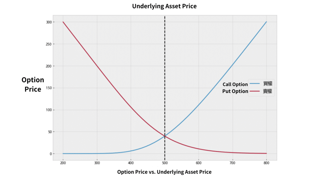
Then, ceteris paribus, we can visualize the relationship between underlying asset price and delta. The financial meaning of delta refers to the amount by which the price of an option increases or decreases when the underlying asset price increases by one unit. From picture down below, It can be observed that when the option is deep out-of-the-money, the delta of both call and put tends towards zero. When the option is deep in-the-money, the delta of the call tends towards one while the delta of the put option tends towards negative one. This indicates that small changes in the underlying asset price have little impact on the options price when it is deep out-of-the-money, while small changes in the underlying asset price can cause significant fluctuations in the option price when it is deep in-the-money and the magnitude of the fluctuations is roughly equal to that of the underlying asset.
s0 = np.linspace(200,800)
k = 500
r = 0.00
sigma = 0.2
T = 252/252

mybs = BS_formula(s0, k, r, sigma, T)
c, p = mybs.BS_delta()

fig = plt.figure(figsize = (12,8))
plt.plot(s0, c, label = '買權')
plt.plot(s0, p, label = '賣權')
plt.axvline(x = 500, color = 'black', linestyle = '--')
plt.axhline(y = 0, color = 'black', linestyle = '--')
plt.xlabel('標的物價格', fontsize = 15)
plt.ylabel('Delta值', fontsize = 15)
plt.title('Delta值 VS. 標的物價格', fontsize = 20)
plt.legend(fontsize = 14)
plt.savefig('black scholes put call delta.png')
plt.show()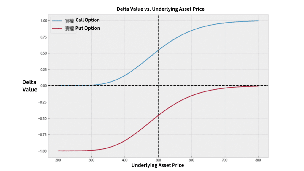
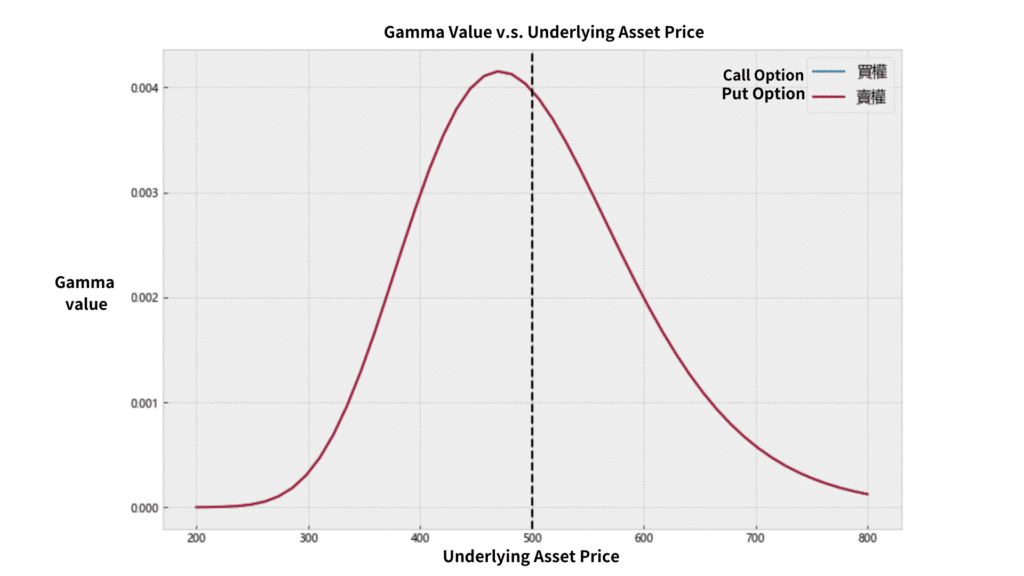
Gamma is the second-order partial derivative of call price with respect to underlying asset price, it can be understood as the slope of delta curve. Ceteris paribus, we can visualize the relationship between underlying asset price and gamma. The gammas of call and put are actually the same, both reach to maximum during at-the-money. That means the magnitude of incremental of delta first accelerate then decelerate, when the underlying asset price moves from deeply out-of-the-money to deeply in-the-money. Code is shown at the end of article.
Moreover, we can observe the change of gamma under different moneyness and time to maturity. A fun fact can be discovered that while in-the-money and approaching to maturity, gamma surges incredibly. And that is the well-known gamma risk. Gamma risk means that while approaching to maturity, the price volatility of options at-the-money usually is usually large. Therefore, most more risk-averting investors try to offset the positions while approaching to maturity. However, some investors might do it inversely, they may long positions before maturity and expect to earn a more decent risk premium.
s0, s1, s2 = 400, 500, 600
k = 500
r = 0.00
sigma = 0.2
T = np.linspace(1, 0.01)

mybs0 = BS_formula(s0, k, r, sigma, T)
c0, p0 = mybs0.BS_gamma()

mybs1 = BS_formula(s1, k, r, sigma, T)
c1, p1 = mybs1.BS_gamma()

mybs2 = BS_formula(s2, k, r, sigma, T)
c2, p2 = mybs2.BS_gamma()

fig = plt.figure(figsize = (12,8))
plt.plot(T, c0, label = '買權(價外)')
plt.plot(T, c1, label = '買權(價平)')
plt.plot(T, c2, label = '買權(價內)')
plt.xlabel('剩餘時間', fontsize = 15)
plt.ylabel('Gamma值', fontsize = 15)
plt.title('Gamma值 VS. 剩餘時間', fontsize = 20)
plt.legend(fontsize = 14)
plt.axis([1.005, -0, -0.005, .045])
plt.savefig('black scholes put call gamma2.png')
plt.show()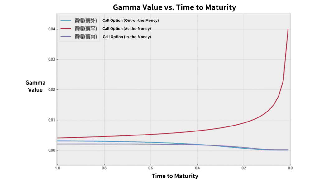
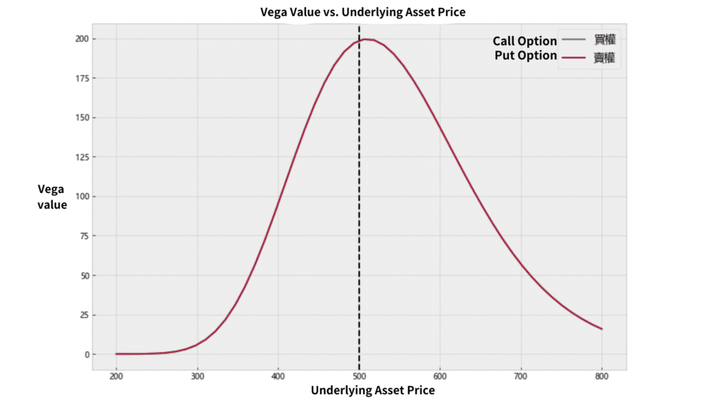
Similar to gamma, the vega of call and put are exactly the same. The meaning of vega refers to the amount by which the price of an option increases or decreases when the volatility of underlying asset price increases by one unit. From below graph, it can be discovered that vega reach to the maximum during at-the-money. That is, the price of options is most sensitive to volatility during at-the-money. Code is shown in the end of article.
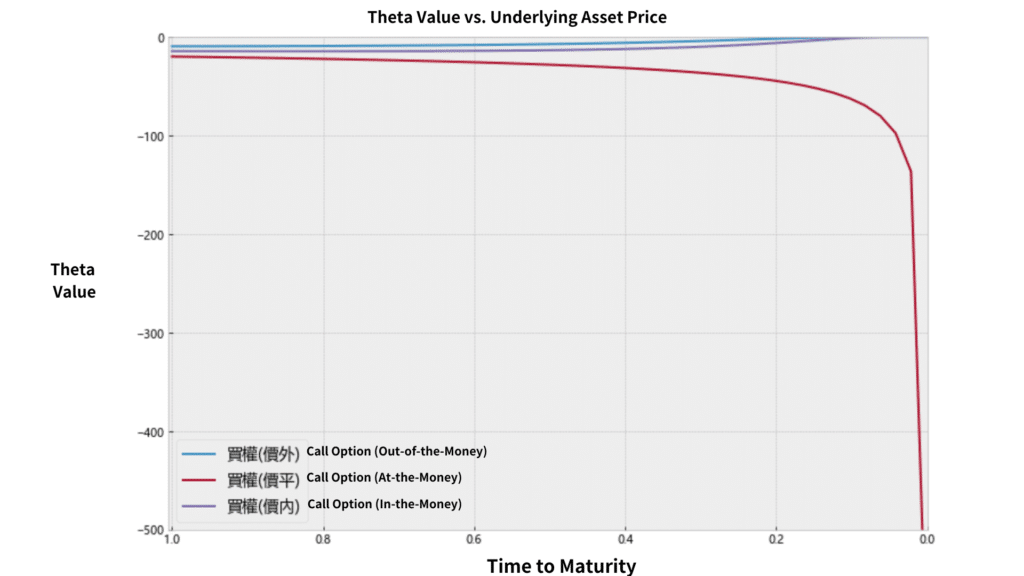
The meaning of theta is the amount by which the price of an option increases or decreases when the time to maturity increases by one unit. We can visualize the relationship between theta and time to maturity. We can see that during deeply in-the-money and out-of-the-money, theta would approach to zero while approaching to maturity. On the contrary, there is a steep downward movement when at-the-money. Moreover, theta is always negative, because as the time moves, the time value of options gradually declines. Code is shown in the end of article.
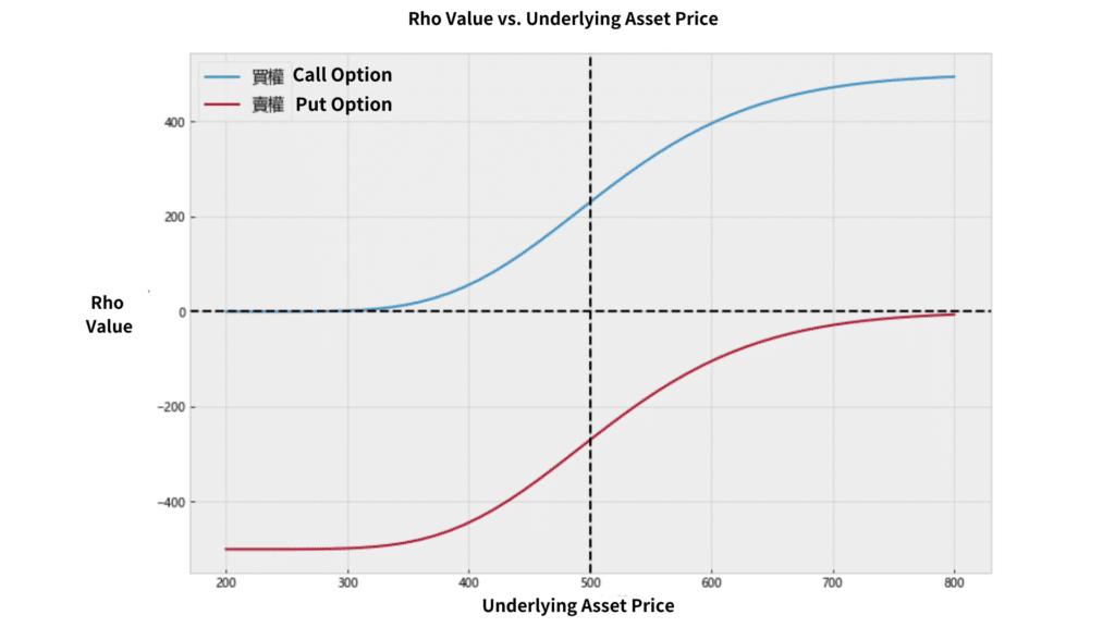
Eventually, rho represents the amount by which the price of an option increases or decreases when the risk-free rate increases by one unit. Also we plot the below curve to observe the relationship between rho and underlying asset price. Since the underlying asset price increase, rho becomes larger. Code is shown in the end of article.
Last but not least, we take the TAIEX call options for example, calculating the theoretical call price at a strike price of 15500, time to maturity of 6 days.
r = 0.012
s0 = stocks.loc['2023-04-10']['收盤價(元)']
k = 15500
sigma = stocks.loc['2023-04-10']['移動報酬波動度']*np.sqrt(252)
T = 6/252

mybs = BS_formula(s0, k, r, sigma, T)
c, p = mybs.BS_price()
c_delta, p_delta = mybs.BS_delta()
c_gamma, p_gamma = mybs.BS_gamma()
c_vega, p_vega = mybs.BS_vega()
c_theta, p_theta = mybs.BS_theta()
c_rho, p_rho = mybs.BS_rho()

print('==2023-04-10履約價為525的台積電買權==')
print('當前標的物價格為 %.3f, 年化波動度為 %.3f, 剩餘期間為 %.3f'%(s0, sigma, T*252))
print('買權理論價格: %.4f, 賣權理論價格: %.4f' %(c,p))
print('買權delta: %.4f, 賣權delta: %.4f' %(c_delta,p_delta))
print('買權gamma: %.4f, 賣權gamma: %.4f' %(c_gamma,p_gamma))
print('買權vega: %.4f, 賣權vega: %.4f' %(c_vega,p_vega))
print('買權theta: %.4f, 賣權theta: %.4f' %(c_theta,p_theta))
print('買權rho: %.4f, 賣權rho: %.4f' %(c_rho,p_rho))
options.loc['2023-04-10'] # 實際買權價格
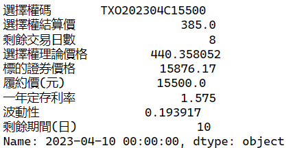
Comparing the theoretical price we calculated with the strike price, we can see that there is a significant difference (435.54–385), indicating that the call option may be undervalued at this moment. In addition, TEJ API also provides a theoretical pricing service in the derivatives financial product database. The theoretical price calculated by TEJ API has a slight difference from ours (440.36 v.s. 435.54), which may be due to different methods of calculating historical volatility or using different risk-free interest rate standards.
The Black-Scholes model remains a foundational tool in options pricing, offering analytical clarity and practical utility through its associated Greeks. By quantifying how option prices respond to market variables, investors and professionals can better understand and manage risk exposure. However, even the most elegant model relies on accurate inputs — and that’s where high-quality market data becomes indispensable. Whether for pricing, hedging, or simulation, TEJ Market Data offers the historical depth and real-time granularity needed to power your quantitative strategies with confidence.
