
Table of Contents
Investments always come with risks, and not all are inevitable. Through risk diversification, the distribution of different asset types could help investors efficiently manage risk and reduce the influence of market volatility on their portfolios. Today’s article will mainly discuss how to use data, comparing the similarity of funds from a scientific point of view.
This article uses Mac OS as a system and jupyter as an editor.
# 載入所需套件
import pandas as pd
import re
import numpy as np
import tejapi
import plotly.graph_objects as go
import random
import seaborn as sns
import math

# 登入TEJ API
api_key = 'YOUR_KEY'
tejapi.ApiConfig.api_key = api_key
tejapi.ApiConfig.ignoretz = Truefund = tejapi.get('TWN/AATT',
paginate = True,
opts = {
'columns':['coid', 'mdate', 'isin',
'fld006_c', 'fld007_c',
'fld014_c','fld015',
'fld016_c','un_name_c',
'risk', 'main_flag',
'fld021', 'currency', 'aunit1',
]
}
)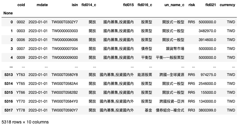
In this article, we will use following columns.
Because most of the columns’ data types are strings, we must encode them to ordinal numbers. Typically, we can simply use ordinal encoding packages to do so; however, we want to make sure that the information on the relative risk of each type can be preserved in sequence, so in this part, we will define our own function to ensure that this information wouldn’t miss.
In order to know how many ordinal numbers should be given, we print out all unique targets in our data frame.
fund["fld016_c"].unique()
style = {
    '':0,
    '保本型': 1,
    '貨幣型': 2,
    '債券型': 3,
    '平衡型': 4,
    'ETF': 5,
    '指數型基金': 6,
    '基金': 7,
    '多重資產': 8,
    '股票型': 9,
    '房地產': 10,
    '產證券化': 11,
    '不動產證券化': 12,
    '科技股': 13,
    '小型股資': 14,
    '能源股票': 15,
    '期貨商品': 16,
}

risk = {
    "":0,
    "RR1":1,
    "RR2":2,
    "RR3":3,
    "RR4":4,
    "RR5":5,
}

area = {
    "國內募集,投資國內":1,
    "國內募集,投資國內外":2,
    "國外募集,投資國內":3,
}

OorC = {
    "封閉":0,
    "開放":1,
}

# adjust sting data to Ordinal encoding data
fund_adj = fund.copy()
fund_adj["fld015"] = fund_adj["fld015"].apply(lambda x: area.get(x))
fund_adj["fld016_c"] = fund_adj["fld016_c"].apply(lambda x: style.get(x))
fund_adj["risk"] = fund_adj["risk"].apply(lambda x: risk.get(x))
fund_adj["fld014_c"] = fund_adj["fld014_c"].apply(lambda x: OorC.get(x))
Next, because we need to visualize the similarity of funds by the diagram, we will rescale the value of “Initial asset size‘‘ by normalization. After normalization, the size value will be rescaled from 0 to 17 since the maximum of the ordinal number is 16. Now “Initial asset size‘‘ no longer contains an actual monetary value; it just reflects the ratio.
# min-max normalization
size = np.array(fund_adj["fld021"].fillna(0))
size = (size - size.min()) / (size.max() - size.min())*len(style)
fund_adj["fld021"] = size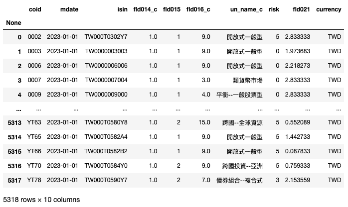
We select the funds whose “currency” is “TWD” to demonstrate visualization, choosing a radar chart to show the difference of funds.
Let’s just randomly pick ten funds to generate the chart.
fund = fund[fund["currency"].str.contains("TWD")]

# randomly pick 10 funds
# set the random state
isin_lst = list(fund["isin"].unique())

random.seed(1)
random_isin_lst = random.sample(isin_lst, 10, )

check_lst = random_isin_lst
categories = ['開放型基金/封閉型基金','募集地及投資區域','投資標的',
              '風險', '成立資產']

fig = go.Figure()
data_lst = []
for num, isin in enumerate(check_lst):

    data = list(fund_adj[fund_adj["isin"] == isin][["fld014_c", "fld015", "fld016_c", "risk", "fld021"]].iloc[0, :])
    data_lst.append(data)

    fig.add_trace(go.Scatterpolar(
          r=data,
          theta=categories,
          fill='toself',
          name=isin
    ))


fig.update_layout(
  polar=dict(
    radialaxis=dict(
      visible=True,
      range=[0, len(style)]
    )),
  showlegend=True
)

fig.show()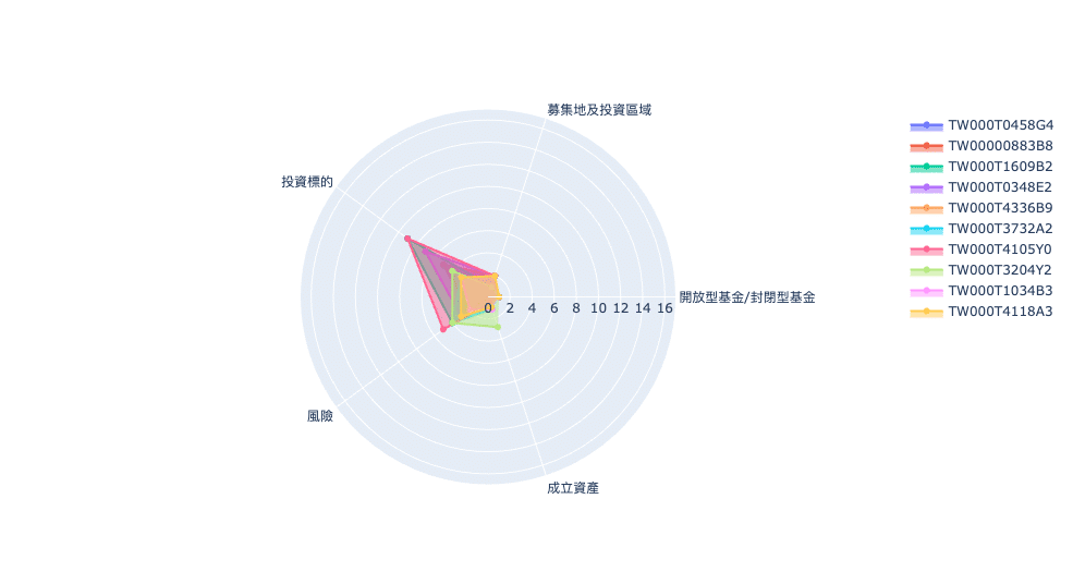
A radar chart can readily and clearly help us understand the difference among funds, but it can not offer us a specific value of how similar they are. Hence, in the next part, we will use the Euclidean distance and the Cosine Similarity to solve this problem.
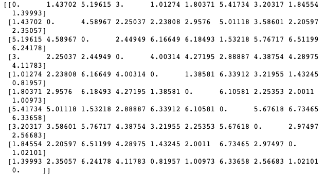
The Euclidean distance is a common way to measure the straight distance of any two points in multi-dimensions; webuild The Euclidean distance formula via Python.
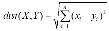
# calculate Euclidean Distance of each couple funds
ED_matrix = np.empty(shape=[len(random_isin_lst), len(random_isin_lst)])
for i in range(len(data_lst)):
for j in range(len(data_lst)):
dist = math.dist(data_lst[i], data_lst[j])
ED_matrix[i, j] = round(dist,5)
print(ED_matrix)
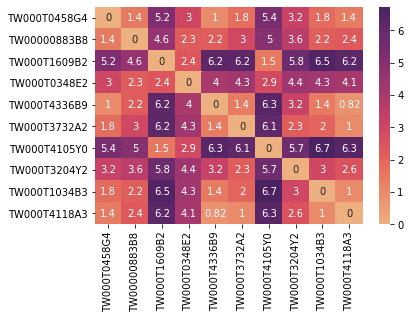
sns.heatmap(ED_matrix, xticklabels = random_isin_lst, yticklabels = random_isin_lst, annot=True, cmap = "flare")By doing so, we already complete the calculation of the Euclidean Distance. However, it is not easy to read the result when it presents as a matrix. We introduce another chart, “heatmap,” to make it better.
Without standardization or normalization, the value of the Euclidean distance doesn’t have a maximum, and the minimum is 0, which means totally the same. And the larger value, the longer distance between the two elements, representing the degree of discrepancy of funds. In the heatmap, the x-axis and y-axis are ISIN codes, and the diagonal from upper-left to lower-right match two same ISIN codes, so the distance will always be 0.
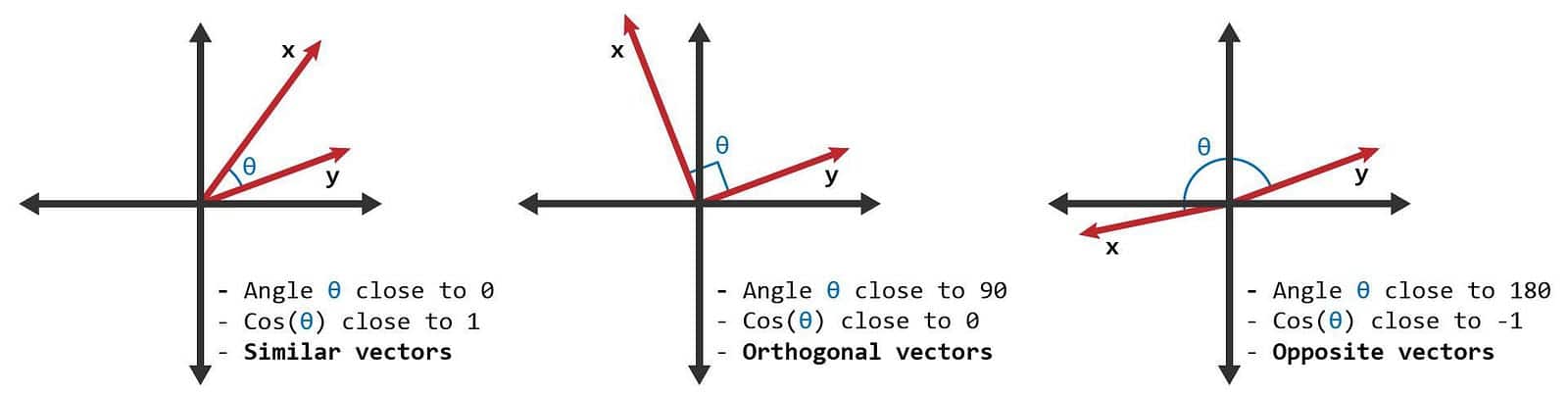
Cosine Similarity evaluates how much any two are similar by measuring two vectors’ cosine values. The cosine value will locate between 1 and -1. 0-degree angle’s cosine value is 1, representing absolutely identical. The cosine value could indicate whether two vectors point in the same direction.
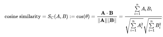
Let’s codify the formula. The method is as same as what we did to the Euclidean distance. A thing worth talking about is that the Cosine Similarity won’t change by the size of the vector because the formula of the Cosine Similarity, fortunately, has a process that acquires the same function as normalization.
# The measure of cosine similarity will not be affected by the size of the vector
CS_matrix = np.empty(shape=[len(random_isin_lst), len(random_isin_lst)])
for i in range(len(data_lst)):
    for j in range(len(data_lst)):
        A = np.array(data_lst[i])
        B = np.array(data_lst[j])
        cosine = np.dot(A,B)/(norm(A)*norm(B))
        CS_matrix[i, j] = round(cosine,5)
print(CS_matrix)
sns.heatmap(CS_matrix, xticklabels = random_isin_lst, yticklabels = random_isin_lst, annot=True, cmap = "flare_r")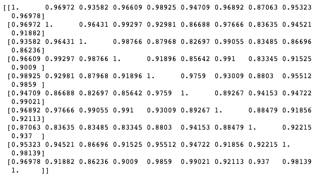
At this point, observant friends should have noticed that the Euclidean distance is smaller for more similar values, while cosine similarity is larger for more similar values. They exhibit an inverse relationship, so when presenting them in a heatmap, it is more convenient to reverse the color scheme for comparing the two calculation results. Therefore, in the visualization code for Euclidean distance, the cmap = “flare” should be changed to cmap = “flare_r”.
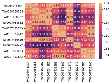
Comparing the two images, the overall distribution trends correspond to each other. In fact, the Euclidean distance is equivalent to cosine similarity.
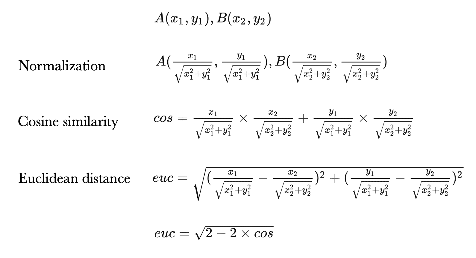
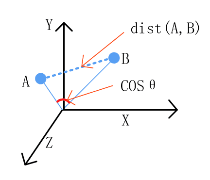
Let’s assume there are two points in space: A and B. By normalizing A and B separately, we obtain unit vectors. The cosine similarity between the two unit vectors can be calculated, and since the denominator is 1, it can be omitted in this case. We can also calculate the Euclidean distance between the two unit vectors and simplify the equation to prove the equivalence.
So, what is the difference between Euclidean distance and cosine similarity?
For Euclidean distance, it calculates the straight-line distance between two points. Therefore, when the trends of the two points are similar, but their vector lengths differ, the Euclidean distance cannot reflect this similarity. For example, in this implementation, if two funds have a high degree of similarity, but one fund has a more significant asset size. In comparison, the other has a smaller size, the Euclidean distance will still show a large discrepancy due to the difference in asset size.
On the other hand, cosine similarity calculates the cosine of the angle between two vectors. Therefore, if two funds have a similar nature, their angle will be small, effectively indicating their similarity.
In the comparison results of similarity, we can observe that the majority of domestic funds exhibit a very high level of similarity. This is likely due to the fact that the current implementation only considers some basic information about the funds, reflecting their initial states when they were established. Readers have the flexibility to incorporate additional information for their calculations, such as returns, expense ratios, and more. TEJ API provides comprehensive fund data and various access methods, allowing readers to customize their own comparison modules according to their preferences.
Please note that this introduction and the underlying asset are for reference only and do not represent any recommendations for commodities or investments. We will also introduce the use of TEJ’s database to construct various option pricing models. Therefore, readers interested in options trading are welcome to purchase relevant solutions from TEJ E-Shop and use high-quality databases to construct pricing models that are suitable for them.
● 【Data Analysis】GRU and LSTM
● 【Quant】Black Scholes model and Greeks
