
Table of Contents
Employee turnover rate refers to the fluctuations in the workforce of a company due to employee departures and new hires within a specific period. This metric is an important concept for assessing the stability of an organizational workforce. A lower employee turnover rate indicates relatively fewer personnel changes within the company, reflecting internal stability and continuity. Conversely, a higher turnover rate may suggest organizational issues, job dissatisfaction, or other factors that could have a negative impact on business operations and the work environment.
Monitoring employee turnover rates can help companies understand and evaluate the effectiveness of their human resource management strategies and take appropriate measures to improve employee retention and satisfaction. This ensures long-term stability and development of the organization. Predicting employee turnover rates allows companies to better plan and manage their human resources, reduce costs, improve talent retention, and enhance organizational efficiency.
This article utilizes the MacOS operating system and Jupyter Notebook as the editor.
#Loading Required Packagesimport pandas as pd import numpy as np import tejapi from collections import Counter from sklearn.model_selection import train_test_split from sklearn.linear_model import LinearRegression import statsmodels.regression.linear_model as sm import matplotlib.pyplot as plt # Log in TEJ API api_key = 'YOUR_KEY' tejapi.ApiConfig.api_key = api_key tejapi.ApiConfig.ignoretz = True
The fields used in this implementation are as follows. Please note that “violate_times” is not an original field in the data table; it is generated after preprocessing.
gte, lte = '2021-01-01', '2021-12-31'
TR = tejapi.get('TWN/ACSR01A',
                   paginate = True,
                   mdate = {'gte':gte, 'lte':lte},
                  )

gte, lte = '2020-01-01', '2021-01-01'
ED = tejapi.get('TWN/AXEMPA',
                   paginate = True,
                   mdate = {'gte':gte, 'lte':lte},
                  )

gte, lte = '2020-01-01', '2021-01-01'
LAW = tejapi.get('TWN/ACSR20A',
                   paginate = True,
                   mdate = {'gte':gte, 'lte':lte},
                  )

gte, lte = '2021-01-01', '2021-12-31'
TWSE = tejapi.get('TWN/ACSR19A',
                   paginate = True,
                   mdate = {'gte':gte, 'lte':lte},
)We filter the columns needed from the education level and TWSE Corporate Governance Evaluation tables and calculate the number of violations of the Labor Standards Act. Next, since the company codes in the TWSE Corporate Governance Evaluation table are in numeric format, which could lead to merging errors, we need to convert them into string type.
ED = ED[["coid", "apct", "bpct" ,"cpct", "dpct", "epct", "fpct" , "emp_sum"]]
LAW = pd.DataFrame(data = [Counter(LAW["coid"]).keys(), Counter(LAW["coid"]).values()]).T.rename(columns = {0:"coid", 1:"violate_times"})
TWSE = TWSE[["coid", "rating"]]
TWSE["coid"] = TWSE["coid"].astype(str)df_main = TR
for i in [ED, TWSE, LAW]:
df_main = pd.merge(df_main, i, on = "coid")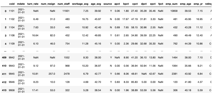
Due to the presence of missing values in the dataset, which could hinder the training of the regression model, it’s important to note that filling missing values with zeros may not always be the best approach. There are various methods for handling missing values depending on the nature of the data and the desired outcomes. However, since the focus of this implementation is on model building, we will fill missing values with zeros for computational convenience.
Furthermore, we will convert the governance rating from string format to numeric format to align with the input requirements of the regression analysis model.
X = dataset_regression.iloc[:, 3:].values
y = dataset_regression.iloc[:, 2].valuesWe split the data into a training set and a test set in an 8:2 ratio and set a random_state to ensure consistent results each time the model is executed.
After feeding the test set into the model, we compare the actual values with the model’s predictions.
x_train, x_test, y_train, y_test= train_test_split(X, y, test_size=0.8, random_state=42) regressor = LinearRegression()#Create an object named 'regressor'.regressor.fit(x_train, y_train)#Train a Linear Regression Modely_pred = regressor.predict(x_test) print(y_pred.shape)#y_predFor a one-dimensional vectornp.set_printoptions(precision = 2)#Displaying two decimal placesP_vs_T = np.concatenate((y_pred.reshape(len(y_pred),1),y_test.reshape(len(y_test),1)),1) print(P_vs_T) #Convert y_pred and y_test to 2D arrays with dimensions (len(y_pred), 1) and then merge them.
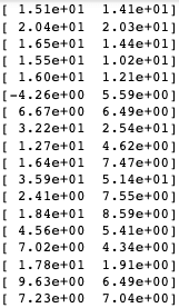
By observing the values, it can be noted that some predicted values have significant errors, and there are even negative values. To gain a clear understanding of the accuracy of the numerical predictions, we will use a bar chart for easy visualization. Additionally, we define predictions as inaccurate when they differ from the actual values by more than 2%.
classification = [1 if abs(x-y)>1 else 0 for x,y in P_vs_T ]
print(Counter(classification))
plt.bar(x = [0,1], height = Counter(classification).values(),tick_label=["False", "True"] )
plt.show()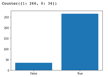
However, through the chart, we can observe that the overall performance of the model is quite good, with an accuracy of 88%.
#Output Model Intercept and Coefficientsprint(regressor.fit(x_train,y_train).intercept_) print(regressor.fit(x_train,y_train).coef_)

Backward elimination is a feature selection method used to exclude features from a model that have no significant impact on the target variable. It starts with the initial full model and gradually removes the features that have the least impact on the model’s performance in each step, until the remaining features meet a certain criterion, such as a significance level (typically when the p-value is less than 0.05). This approach helps prevent overfitting, reduces model complexity, and improves the interpretability and predictive power of the model. Backward elimination is widely used in multiple linear regression to select the most influential features for the target variable.
The choice of the significance level, why it’s typically set at p-value < 0.05, and the concept of hypothesis testing:
Backward elimination involves hypothesis testing, which is a statistical method used to make inferences about population parameters based on sample data. In hypothesis testing, two opposing hypotheses are proposed: the null hypothesis and the alternative hypothesis. The null hypothesis typically represents no effect, no difference, or no association, while the alternative hypothesis represents an effect, a difference, or an association.
Through the collection of sample data and statistical analysis, a test statistic is calculated to assess the support for or against the null hypothesis. By comparing the value of the test statistic to a predefined significance level, we make a statistical judgment about the results. If the test statistic’s value deviates significantly from what would be expected under the null hypothesis, we may reject the null hypothesis and support the alternative hypothesis. Otherwise, we fail to reject the null hypothesis.
The p-value represents the probability of obtaining the observed results or more extreme results when the null hypothesis is true. When the p-value is less than the predefined significance level (typically 0.05), we can reject the null hypothesis. This is because a p-value less than 0.05 indicates that the observed results are very rare, given the assumptions of the null hypothesis. Thus, rejecting the null hypothesis means that we have sufficient evidence to support the alternative hypothesis.
However, it’s important to note that 0.05 is just a commonly used significance level. In some cases, a more stringent significance level (e.g., 0.01) may be chosen based on the nature of the study or the severity of the issue. Additionally, other factors such as sample size, study design, and effect size should be considered when making appropriate statistical judgments and interpreting results. Rejecting the null hypothesis is only one part of statistical inference and should be interpreted and reported with caution to avoid overinterpretation or misleading conclusions.
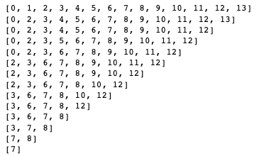
In our case, we use a for loop to progressively eliminate parameters while retaining the model information with the highest accuracy.
#Adding a Constant of 1 to Comply with the Regression Modely = b0+b1*X+b2*X^2+b3*X^3... x_train = np.append(arr = np.ones((len(x_train[:,1]),1)).astype(int), values = x_train, axis = 1) # back elimination col = [0,1,2,3,4,5,6,7,8,9,10,11,12,13] R_square = [] for i in range(len(col)): x_opt=np.array(x_train[:,col], dtype=float) regressor_OLS=sm.OLS(endog=y_train, exog= x_opt).fit() R_square.append(regressor_OLS.rsquared) if regressor_OLS.rsquared == max(R_square): summary = regressor_OLS.summary() attribute = col.copy() P = regressor_OLS.pvalues.tolist() print(col) col.pop(P.index(max(P)))
We will visualize the R-squared values after eliminating parameters each time with a line chart. R-squared is a statistical measure used to assess the extent to which a regression model explains the variability of the dependent variable. It indicates the percentage of the variance in the dependent variable that can be explained by the independent variables in the model. R-squared values range from 0 to 1, where values closer to 1 indicate that the model can better explain the variability of the dependent variable, and values closer to 0 indicate weaker explanatory power of the model. Specifically, an R-squared of 0 means the model cannot explain the variance in the dependent variable, while an R-squared of 1 indicates that the model fully explains the variance in the dependent variable.
plt.plot(R_square,'ro--', linewidth=2, markersize=6)
plt.xticks(ticks = [i for i in range(0,14)], labels= [i for i in range(1,15)][::-1])

plt.title("change in R_square")
plt.xlabel('number of attribute')
plt.ylabel('R_square')

plt.show()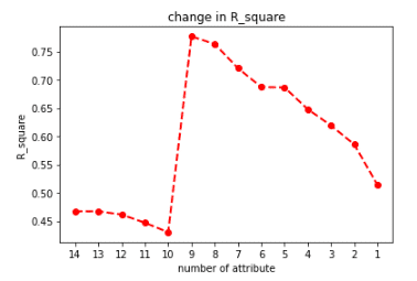
We extract the parameters corresponding to the highest R-squared value and print out the names of the corresponding columns.
col_map = dict(zip([0,1,2,3,4,5,6,7,8,9,10,11,], dataset_regression.iloc[:, 3:].columns))

print(attribute)
print(list(map(lambda x:col_map.get(x), attribute)))
Viewing Statistics for the Highest R-squared
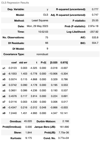
In conclusion, through reverse elimination, we successfully improved the model’s accuracy from an initial 46% to 77%. By analyzing the composition of parameters, we found that employee turnover is primarily influenced by factors such as years of service, salary, and the proportion of employees with education levels below a college degree. However, these conclusions are based on statistical principles, and the interpretation of the R-squared value should be combined with specific context and the characteristics of the model. It can help assess the model’s fitness and predictive capability and compare the strengths and weaknesses of different models. Therefore, it is essential to use R-squared cautiously and integrate it with other evaluation metrics and expert judgment for a comprehensive analysis to fully understand the model’s explanatory power and limitations.