To construct a portfolio based on Jim Slater’s principle

Table of Contents
Jim Slater is one of the well-known U.K. investors. He used to write column articles of portfolio recommendation for Sunday Telegraph and was famous for earning around 68.9% return during the period between 1963 to 1965, while the U.K. stock market only grew at 3.6% at the same period. Jim Slater’s ‘Zulu Principle’ stresses the importance of focusing on your own niche field, where you can take advantage of. Therefore, Jim Slater especially pays attention to small and medium size firms that have long-term profit growth and relative strength and adopts price/earnings to growth ratio (PEG ratio) as an important standard for valuation, as the following shown:
We use Windows OS and Jupyter Notebook in this article
import pandas as pd
import numpy as np
import tejapi
import matplotlib.pyplot as plt
tejapi.ApiConfig.api_key = "Your Key"
tejapi.ApiConfig.ignoretz = True
Since Jim Slater’s stock-picking standards include some subjective judgement factors, we present the following objective and quantitative indicators based on them and also adjust them by considering Taiwan stock market environments
Condition1: Firm market value < Market average market value
Condition2: Positive net incomes in the past five years
Condition3: Net income growth > 15% in three consecutive years
Condition4: Expected net income growth ≥ 15%
Condition5: 5-year average cash flow from operating > 5-year average net income
Condition6: Recent cash flow from operating > recent net income
Condition7: Recent operating margin ≥ 10%
Condition8: Recent return on capital employed ≥ 10%
Condition9: Recent debt/equity ratio < 50%
Condition10: Recent shareholding ratio of directors and supervisors ≥ 20% or recent increase in this ratio
Condition11: Expected PE ratio ≤ 20
Condition12: Expected PE ratio/Expected net income growth ≤ 1.2
Condition13: Monthly excess return > 0
Step 1. Obtain the codes of TSE listed common stocks
security = tejapi.get('TWN/ANPRCSTD',
                     paginate = True)
stock_list = security[(security['mkt'] == 'TSE') & (security['stype'] == 'STOCK')]['coid'].tolist()

Step 2. Obtain all the data we need and create condition column
#container for outputs
data = pd.DataFrame()

for coid in stock_list:
    #Obtain financial data
    finance = tejapi.get('TWN/AIM1A',
                    coid = coid,
                    mdate = {'gte':'2000-01-01'},
                    opts = {'pivot':True, 'columns':['coid','mdate','MV','R531','R405','7210','R106','2402','0010','1100','R504']},
                    paginate = True,)
    #Select data in December to annualize the data
    finance = finance[finance['mdate'].dt.month == 12].reset_index(drop=True)

    #Add 'match year' column for the later combination purpose
    finance['MatchYear'] = finance['mdate'].dt.year

    #Calculate expected net income growth by using 5-year moving average of net income growth
    finance['ExpectedNetIncomeGrowth'] = finance['R531'].rolling(5).mean()

    #Calculate 5-year moving average of cash flow from operating activities
    finance['5_YearAverageOperatingCashFlow'] = finance['7210'].rolling(5).mean()

    #Calculate 5-year moving average of net income
    finance['5_YearAverageNetIncome'] = finance['R531'].rolling(5).mean()

    #Condition2: Positive net incomes in the past five years
    finance['positive_profit'] = np.where(finance['R531'] > 0, 1, 0)
    finance['condition2'] = np.where(finance['positive_profit'].rolling(5).sum() == 5, 1, 0)

    #Condition3: Net income growth > 15% in three consecutive years
    finance['net_income_growth_higher_than_15'] = np.where(finance['R405'] >= 15, 1, 0)
    finance['condition3'] = np.where(finance['net_income_growth_higher_than_15'].rolling(3).sum() == 3, 1, 0)

    #Condition4: Expected net income growth ≥ 15%
    finance['condition4'] = np.where(finance['ExpectedNetIncomeGrowth'] >= 15, 1, 0)

    #Condition5: 5-year average cash flow from operating > 5-year average net income
    finance['condition5'] = np.where(finance['5_YearAverageOperatingCashFlow'] > finance['5_YearAverageNetIncome'], 1, 0)

    #Condition6: Recent cash flow from operating > recent net income
    finance['condition6'] = np.where(finance['7210'] > finance['R531'], 1, 0)

    #Condition7: Recent operating margin ≥ 10%
    finance['condition7'] = np.where(finance['R106'] >= 10, 1, 0)

    #Condition8: Recent return on capital employed ≥ 10%
    finance['ROCE'] = (finance['2402']/(finance['0010']-finance['1100']))*100
    finance['condition8'] = np.where(finance['ROCE'] >= 10, 1, 0)

    #Condition9: Recent debt/equity ratio < 50%
    finance['condition9'] = np.where(finance['R504'] < 50, 1, 0)

    #Remove NaN data
    finance = finance.dropna().reset_index(drop=True)

    #Obtain shareholding ratio data
    chip  = tejapi.get('TWN/ABSTN1',
                        coid = coid,
                        mdate = {'gte':'2000-01-01'},
                        opts = {'columns':['coid','mdate','fld005']},
                        paginate = True)

    #Check if the latest shareholding ratio of insider increases
    chip['if_shareholding_ratio_increase'] = np.where(chip['fld005'] > chip['fld005'].shift(1),1,0)

    #Select February data, since the latest shareholding data we have at portfolio formation data is February data
    chip = chip[(chip['mdate'].dt.month == 2)].reset_index(drop=True)

    #Condition10: Recent shareholding ratio of directors and supervisors ≥ 20% or recent increase in this ratio
    chip['condition10'] = np.where((chip['fld005'] >= 20) | (chip['if_shareholding_ratio_increase'] == 1),1,0)

    #Add 'match year' column for the later combination purpose, the reason of 'minus 1' is because this ratio data matches last year's financial data
    chip['MatchYear'] = chip['mdate'].dt.year - 1

    #Creat a temporary dataframe by merging finance data with ratio data on firm's code and matchyear
    temp = finance.merge(chip, on = ['coid','MatchYear'])

    #Store this temporary dataframe in data
    data = data.append(temp).reset_index(drop = True)
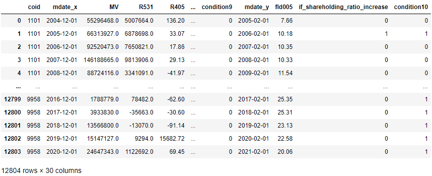
Each loop deals with each stock. Because of the huge amount of data obtained, it takes around 30 ~ 40 minutes. The procedure includes data frequency adjustment, using np.where() to create condition columns, combining data from different databases and storing the outputs in data. Besides, since the index might be disordered after selecting, adding, sorting or removing data, we usually add reset_index(drop=True). The following is the final content of data:
data_cp = data.copy()
To avoid modifying the raw data, we copy data and proceed it with data_cp
#Calculate market average market value
avg_mv = data_cp.groupby(by = 'mdate_x')['MV'].mean()#Map market average market value to data_cp by date column
data_cp['MarketAverageMarketValue'] = data_cp['mdate_x'].map(avg_mv)#Condition1: Firm market value < Market average market value
data_cp['condition1'] = np.where(data_cp['MV'] < data_cp['MarketAverageMarketValue'], 1, 0)
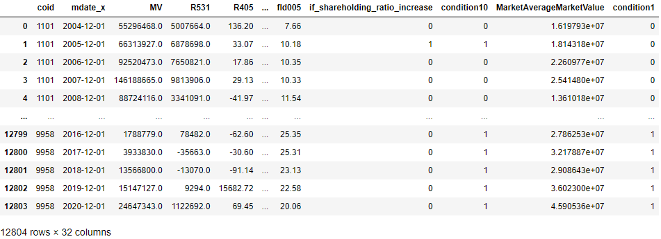
Once we have the market value of whole firms, we can now create condition1 column. Here we use map() to map market average market value to data_cp by its date column.
#We choose the columns we need
data_cp = data_cp[['coid','mdate_x','MV','ExpectedNetIncomeGrowth','condition1','condition2','condition3','condition4','condition5','condition6','condition7','condition8','condition9','condition10']]
#Calculate the score and select those higher than 9
data_cp['score'] = data_cp['condition1'] + data_cp['condition2'] + data_cp['condition3'] + data_cp['condition4'] + data_cp['condition5'] + data_cp['condition6'] + data_cp['condition7'] + data_cp['condition8'] + data_cp['condition9'] + data_cp['condition10']
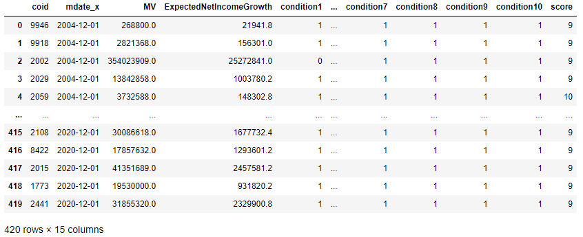
data_cp = data_cp[data_cp['score'] >= 9].sort_values(by = 'mdate_x').reset_index(drop=True)
Step 3. Market-side condition and portfolio return calculation
Panel = pd.DataFrame()    #To store complete data for each stock
Return = pd.DataFrame()   #To store portfolio return
date_list = pd.DatetimeIndex(data_cp['mdate_x'].unique()) #Transform unique date into DatatimeIndex list

for date in date_list:
    #Each year has a dataframe
    table = data_cp[data_cp['mdate_x'].dt.year == date.year].reset_index(drop=True)

    #Get the previous year's PE ratios at portfolio formation date
    stocks = table['coid'].tolist()
    pe_ratio = tejapi.get('TWN/APRCD1',
                             coid = stocks,
                             opts = {'columns':['coid','mdate','per_tse']},
                             mdate = {'gte': date + pd.Timedelta(days = 120 - 365) , 'lte': date + pd.Timedelta(days = 120)},
                             paginate = True)

    #Calculate one-year average PE ratio as expected PE ratio
    pe_estimate = pe_ratio.groupby(by = 'coid').mean().reset_index()

    #Obtain the excess monthly return data
    relative_performance = tejapi.get('TWN/APRCD2',
                             coid = stocks,
                             opts = {'columns':['coid','mdate','rois_m']},
                             mdate = {'gte': date + pd.Timedelta(days = 120 - 5), 'lte': date + pd.Timedelta(days = 120)}, #We just need the data closest to portfolio date
                             paginate = True)

    #Pick the last data for each stock
    relative = relative_performance.groupby(by = 'coid').last().reset_index()

    #Combine expected PE with stock relative performance
    merge = pe_estimate.merge(relative, on = 'coid')

    #Alter column name to combine with table
    merge = merge.rename(columns = {'mdate':'mdate_x', 'per_tse':'ExpectedPE_ratio'})
    merge = table.merge(merge[['coid', 'ExpectedPE_ratio','rois_m']], on = 'coid')

    #Calculate PEG ratio
    merge['PEG_ratio'] = merge['ExpectedPE_ratio']/merge['ExpectedNetIncomeGrowth']

    #Filter by market-side conditions, get the final constituent stocks
    final = merge[(merge['ExpectedPE_ratio'] <= 20)&(merge['PEG_ratio'] <= 1.2) & (merge['rois_m'] > 0)].reset_index(drop=True)

    #Calculate the weight by firm's market value
    final['weight']  = final['MV']/ final['MV'].sum()

    #Obtain return data (including market as benchmark)
    stocks = final['coid'].tolist()
    ret = tejapi.get('TWN/APRCD2',
            coid = stocks + ['Y9997'],
            paginate = True,
            opts = {'columns':['coid','mdate','roi_y']},
            mdate = {'gte': date + pd.Timedelta(days = 120), 'lte': date + pd.Timedelta(days = 120+365)})

    #Period Return: get the last return data of each stock, which is yearly return
    period_ret = ret.groupby(by = 'coid')['roi_y'].last().reset_index()

    #Assign date for later combination
    period_ret['mdate_x'] = date

    #Combine it with final, outer can make sure market return data is not removed
    temp = final.merge(period_ret,on = ['coid','mdate_x'], how = 'outer')

    #Store this year's complete data
    Panel = Panel.append(temp).reset_index(drop=True)

    #Hold the portfolio since 2005(built on 2004 data), 2020 year is excluded because its portfolio hasn't been held for a year
    if 2020 > date.year >= 2004:
        #Calculate portfolio return and market return
        fee = 0.1425*2 + 0.3
        eq_port = temp.loc[:,'roi_y'].values[:-1].mean() - fee           #Equally-weighted portfolio return (excluding market return)
        val_port = (temp['weight']*temp['roi_y']).dropna().sum() - fee   #Market-Cap-weighted portfolio return (excluding market return)
        mkt = temp['roi_y'].values[-1]                                   #Market return
        #Store whole return
        Return = Return.append(pd.DataFrame(np.array([date,eq_port,val_port,mkt]).reshape((1,4)),columns = ['mdate_x','Equally-Weighted Portfolio Return','Market-Cap-Weighted Portfolio Return','Market Return'])).reset_index(drop=True)
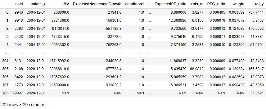
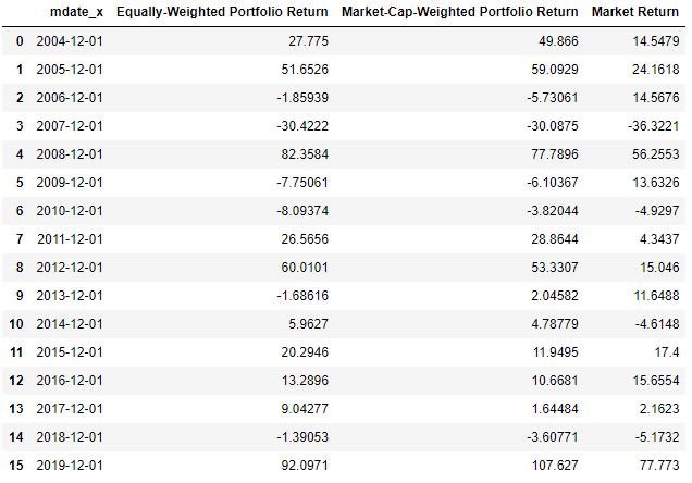
Here we use each year as one loop and make the second filtering by market-side conditions and calculate portfolio return. It’s worth noting that the time window of PE ratio we obtain is the previous year at portfolio formation date. For example, if mdate_x is ‘2020–12–01’, it means we’ll construct the portfolio on ‘2021–03–31’(120 days later) and we need PE ratio from ‘2020–03–31’ to ‘2021–03–31’). Since this portfolio will be held until ‘2022–03–31’ which hasn’t happened yet, we will exclude 2020-based portfolio while calculating portfolio return.
Panel
Return
Step 4. Visualize cumulative return (Code can be found in Source Code)
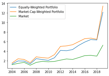
Step 5. Performance (Code can be found in Source Code)

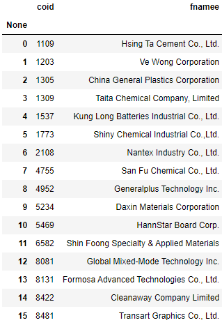
Step 6. Constituent stocks of 2020-based portfolio (Code can be found in Source Code)
Due to the huge data that covers financial, shareholding status and market-side data, we suggest readers begin with fewer firms, shorter time windows or fewer stock selection standards. If the output meets your expectation, then you can examine it from a longer period. In addition to time length, the quality and various data are required. Therefore, we recommend readers to purchase different databases in TEJ E Shop, in order to put those well-known investors’ investing philosophy into practice!
The content of this webpage does not constitute any offer or solicitation to offer or recommendation of any investment product. There may be survivor bias existing since we use current listed companies. It is for learning purposes only and does not take into account your individual needs, investment objectives and specific financial circumstances. Investment involves risk. Past performance is not indicative of future performance. Readers are requested to use their personal independent thinking skills to make investment decisions on their own. If losses are incurred due to relevant suggestions, it will not be involved with the author.