Effective Explanatory Variables for Economic Growth

Table of Contents
Least Absolute Shrinkage and Selection Operator, short as Lasso, is mainly used for variable selection and regularization in Regression. The function of “Penalty” setting would in Lasso lets us adjust the complexity. Therefore, with Lasso, we are able to alleviate “Overfitting”.
Penalty in the model is used to determine the weights between “Error” and “Amount of Variable”. Namely, we would not only consider the goal to minimize error, but try to reduce amount of variable so as to achieve an “adequate” complexity. Hence, if we set a small parameter on penalty, the model will prefer “reducing error”. On the other hand, a large parameter represent that model emphasize “reducing variable amount”.
Note: Penalty parameter must greater than 0 to match the condition of “considering less variables”. To boot, the parameter setting name is “Alpha” in Python package.
MacOS & Jupyter Notebook
# Basic
import numpy as np
import pandas as pd# Graph
import matplotlib.pyplot as plt
%matplotlib inline
import seaborn as sns
sns.set()# TEJ API
import tejapi
tejapi.ApiConfig.api_key = 'Your Key'
tejapi.ApiConfig.ignoretz = True
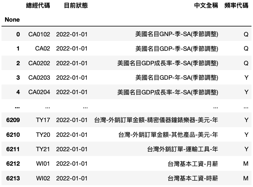
Macroeconomics Data Explain Table: Illustrate information about recorded Macroeconomics data. Code is “GLOBAL/ABMAR”.
Macroeconomics Data Table: Macroeconomics data from official government. Source: IMF, OECD and relatively professional issues. Code is “GLOBAL/ANMAR”.
Step 1. Import Basic Information of Data
factor = tejapi.get('GLOBAL/ABMAR',
                opts={'columns': ['coid','mdate', 'cname', 'freq']},
                chinese_column_name=True,
                paginate=True)
Step 2. Select Specific Data
# Selection
list1 = list(factor['總經代碼'][i] for i in range(0,6214) if '台灣' in factor.iloc[i,2] and factor['頻率代碼'][i] == 'Q')# Table
factor = factor[factor['總經代碼'].isin(list1)].reset_index().drop(columns =['None', '目前狀態', '頻率代碼'])
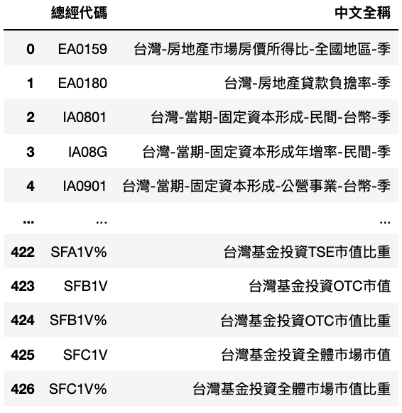
Since the amount of Macro indexes is extremely large and diverse. It is impossible to fit all data in model. As a result, we would only consider ”Quarterly Data of Taiwan”.
Step 3. Import Numeric Data
data = tejapi.get('GLOBAL/ANMAR',
                  mdate={'gte': '2008-01-01', 'lte':'2021-12-31'},
                  opts={'columns': ['coid','mdate', 'val', 'pfr']},
                  coid = list1, # 符合條件的指標
                  chinese_column_name=True,
                  paginate=True)
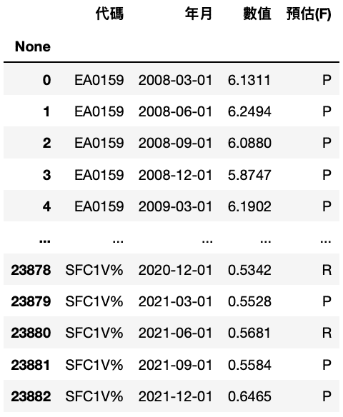
Step 1. Remove Forecasting Data
data = data[data['預估(F)'] != 'F']
Step 2. Rearrange Table
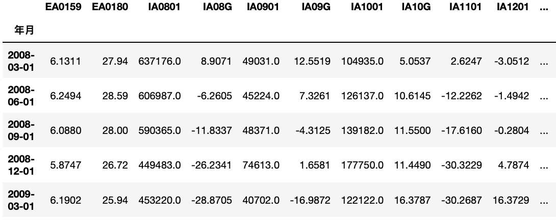
data = data.set_index('年月')df = {}for i in list1:
    p = data[data['代碼'] == i]
    p = p['數值']
    df.setdefault(i, p)df = pd.concat(df, axis = 1)
We firstly set “Year-Month” as table index. Then, read each type of data. Lastly, arrange new table that each columns record different Macro indexes.
Step 3. Select Economic Growth Rate, Y
# Display all economic growth rate indexes
growth_reference = list(factor['總經代碼'][i] for i in range(0,427) if '經濟成長率' in factor.iloc[i,1])factor[factor['總經代碼'].isin(growth_reference)]# Select 'NE0904-季節調整後年化經濟成長率' as Y
growth = df['NE0904']
Since Taiwan is export-oriented, its economic performance is easily affected by global consumption cycle. We, therefore, choose “NE0904-Seasonal Adjusted Annualized Rate(saar)” as the reference of economic growth.
# Remove economic growth data in df
df = df.drop(columns = growth_reference)# Remove nan
df = df.dropna(axis = 1, how = 'any')
Step 4. Stationary Test
from statsmodels.tsa.stattools import adfuller

for i in df.columns.values:
    p_value = adfuller(df[i])[1]
    if p_value > 0.05:
        df = df.drop(columns = i)

df = df.dropna(axis = 1, how = 'any')print('解釋變數量:', len(df.columns))
print('經濟成長率定態檢定P值:', '{:.5f}'.format(adfuller(growth)[1]))
Implement stationary test on each variable with for loop. Remove data which is non-stationary. We would not conduct differencing. On top of that, calculate the amount of explanatory variable, which is 148. Lastly, conduct stationary test on economic growth rate. P-value is 0.0000.
Step 1. Import Packages & split Data
from sklearn.linear_model import Lasso
from sklearn.pipeline import Pipeline
from sklearn.preprocessing import PolynomialFeaturesdf_train = df.head(45)
df_valid = df.tail(10)growth_train = growth.head(45)
growth_valid = growth.tail(10)
Step 2. Model Fitting
We would only show the code of “Big Alpha” model here. As for the code of medium and small alpha model, please check “Source Code”.
# big alpha modelLasso_l = Pipeline(steps = [('poly', PolynomialFeatures(degree = 1)), ('Lasso', Lasso(alpha = 1000))])
large = Lasso_l.fit(df_train, growth_train)
growth_pred_l = large.predict(df_valid)
large_alpha = list(growth_pred_l)print('大Alpha的MSE:', metrics.mean_squared_error(growth_valid, large_alpha))
Due to the amount of explanatory variable, which is 148, we would consider the effectiveness of each variable itself. We make degree as 1. Besides, in order to make model more stricter, we set Alpha with three class, 10, 100 and 1000.
MSE of each model are as follow:
Big Alpha MSE: 207.82
Medium Alpha MSE: 526.29
Small Alpha MSE: 1399.59
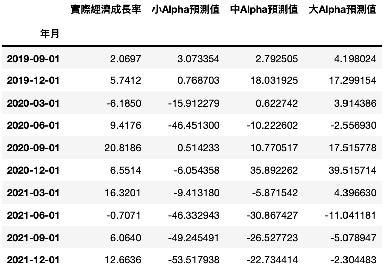
According to above comparison, we would tell that the big alpha model outperforms others. Subsequently, we would visualize valid dataset and select the final model.
Step 1. Rearrange Table
pred_data = {'小Alpha預測值': small_alpha, '中Alpha預測值': medium_alpha, '大Alpha預測值':large_alpha}
result = pd.DataFrame(pred_data, index = growth_valid.index)
final = pd.concat([growth_valid, result], axis = 1)
final = final.rename(columns={'NE0904':'實際經濟成長率'})
Step 2. Visualization
# Make Python apply Chinese
plt.rcParams['font.sans-serif'] = ['Arial Unicode MS']plt.figure(figsize=(15,8))plt.plot(final['實際經濟成長率'])
plt.plot(final['小Alpha預測值'])
plt.plot(final['中Alpha預測值'])
plt.plot(final['大Alpha預測值'])plt.legend(('實際成長率', '小Alpha預測', '中Alpha預測', '大Alpha預測'), fontsize=16)
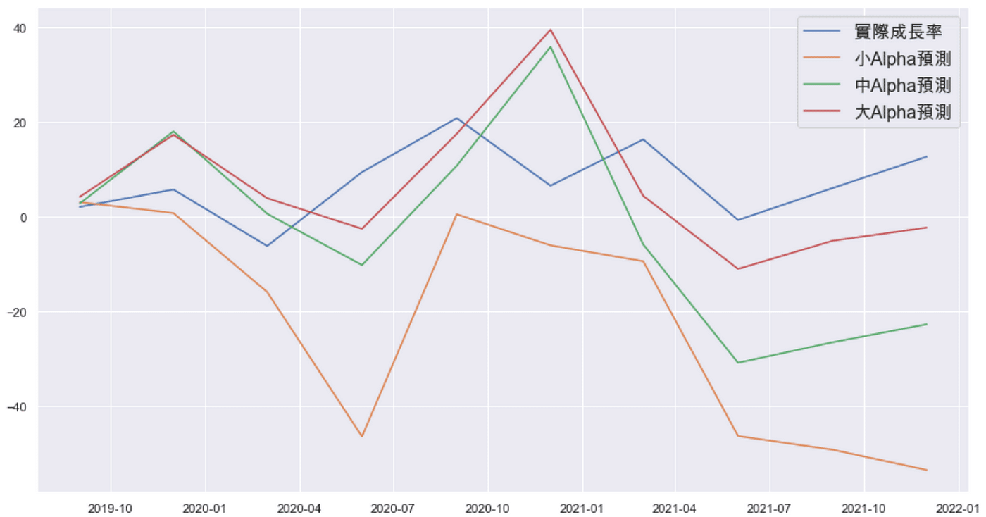
Based on above graph, we could clearly compare the three model, big(red) medium(green) and small(orange) alpha with actual number(blue). We conclude that result of big alpha model is closer to actual one than other two model. Hence, we would apply big alpha model to find effective variable for explaining economic growth rate.
Step 2. Effective Variables
# Re-fitting the model
lasso = Lasso(alpha = 1000)
mdl = lasso.fit(df_train,growth_train)# Display variables that coefficient is larger than 0
lasso_coefs = pd.Series(dict(zip(list(df_valid), mdl.coef_)))
coefs = pd.DataFrame(dict(Coefficient=lasso_coefs))
coid = coefs[coefs['Coefficient'] > 0].index# Match the Code of selected variables to find Chinese name
factor[factor['總經代碼'].isin(coid)]
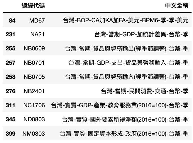
According to above chart, we conclude that the majority of variables consists of international trade-related and finance-related data, which matches the condition of Taiwan, an export-oriented country. To boot, one of above variables is GDP of Education Industry. It proves that the improvement of education among population would benefit economic growth.Therefore, keep cultivating next generation is what we should notice.
With above context, we firstly show data selection and pre-processing. Subsequently, implement model fitting and comparison. Lastly, find the effective explanatory variables for economic growth. It is clear that we spare advanced data transformation or differencing so as to keep this article from redundancy. Of course you do not have to follow our steps. As for the setting of parameters in model, we encourage you to try your own set. Believe you would gain much knowledge by practice. Last but not least, if you are interested in model construction, but concern the data source. Welcome to purchase the plans offered in TEJ E Shop and use the well-complete database to implement your own model.