
Table of Contents
The Average True Range (ATR), an indicator developed by J. Welles Wilder, is designed to assess the extent of price fluctuations within a specific period. ATR is commonly utilized as a tool in technical analysis, assisting traders in understanding the volatility of a particular asset and subsequently determining entry points, exit points, and stop-loss levels for loss aversion purpose.
When the ATR value is high, it indicates that the asset’s price is experiencing more significant fluctuations. Conversely, when the ATR value is low, it signifies that the asset’s price is relatively stable.
This article will use the “Bollinger Bands & ATR Loss Aversion Strategy” as the experimental group and the commonly used “Bollinger Bands” strategy as the control group. The objective is to observe whether the experimental group employing the loss aversion strategy can perform better.
This article is written using Windows 11 and Jupyter Lab as the editor.
import os
import tejapi
import pandas as pd
import numpy as np
import matplotlib.pyplot as pltThe backtesting time period is between 2022–01–01 to 2023–01–01, and we take TSMC(2330) as an example.
# set tej_key and base
tej_key = 'Your Key'
api_base = 'https://api.tej.com.tw'

os.environ['TEJAPI_KEY'] = tej_key
os.environ['TEJAPI_BASE'] = api_base

# set date
start = '2022-01-01'
end = '2023-01-01'

os.environ['mdate'] = start + ' ' + end
os.environ['ticker'] = '2330'

!zipline ingest -b tquantFrom the pipeline and zipline function provided in TQuant Lab, we can:
We executed the configured loss aversion strategy with the trading period from 2022-01-01 to 2022-12-31 and with the initial capital of 10,000,000 NTD. The output shows the portfolio value chart and illustrate the stock price trends of TSMC, along with the Bollinger Bands and buy/sell signals.
Since this article uses an experimental group and a control group to observe the effectiveness of setting stop-loss points, the results of the two groups will be presented separately below to facilitate our loss aversion analysis of the stop-loss effect.
from zipline import run_algorithm

results = run_algorithm(
    start = start_time,
    end = end_time,
    initialize=initialize,
    bundle='tquant',
    analyze=analyze,
    capital_base=1e7,
    handle_data = handle_data
)

results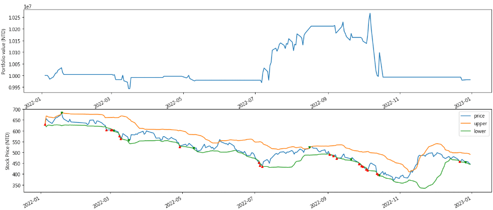
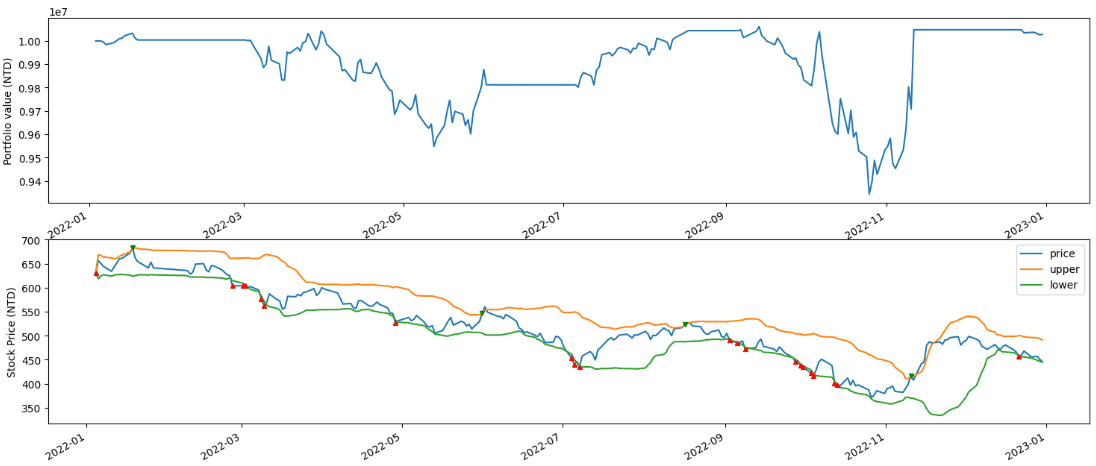
Comparing the experimental group with the control group, it is evident that the asset value of the experimental group incurred only a slight loss due to the implementation of stop-loss points, and the overall assets have room for upward profitability. In contrast, the asset value of the control group mainly experienced losses, with the maximum loss exceeding 6%.
Next, we can observe the timing of stop-loss in the experimental group through the chart of trading entry and exit points (red arrows indicate buying, green arrows indicate selling). Our loss aversion strategy implemented two stop-losses in March, limiting the loss to only 0.5% and effectively avoiding the bearish trend in April and May. Additionally, stop-losses were executed in September and October, when the control group did not carry out stop-loss and continued to average down. Consequently, the control group experienced a gradual reduction in asset value. Although there was a profit from the price spread when exiting, restoring the asset value to the initial level, investors had to endure the downside risk in September and October.
import pyfolio as pf
returns, positions, transactions = pf.utils.extract_rets_pos_txn_from_zipline(results)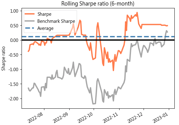
benchmark_rets = results['benchmark_return']On average, the experimental group, which implemented stop-loss, has a Sharpe Ratio of around 0.9, while the control group has only 0.1. Additionally, the Sharpe Ratio of the experimental group remains greater than 0 throughout the backtesting period, whereas the control group once drops to around -0.1.
pf.plotting.plot_rolling_returns(returns, factor_returns=benchmark_rets)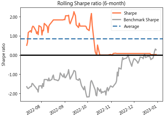
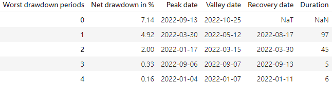
The charts shows that the control group without setting stop-loss experiences more significant drawdowns, with the maximum drawdown reaching 7.14%. In contrast, the experimental group’s maximum drawdown is only 2.8%, and aside from the maximum drawdown, all other drawdowns are less than 1%.
from pyfolio.plotting import show_worst_drawdown_periods
show_worst_drawdown_periods(returns, top=5)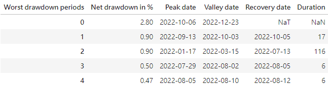
For this implementation, in order to achieve the effect of “loss aversion,” we combined the Bollinger Bands strategy with the Average True Range (ATR) to implement stop-loss. Simultaneously, we used the Bollinger Bands strategy without setting stop-loss as the control group to highlight the effectiveness of the ATR stop-loss.
From the analysis we conducted above, we can see that ATR indeed helps us achieve “loss aversion,” especially during bearish trends, where the establishment of stop-loss points effectively helps us avoid the risk of asset depreciation. Using the Pyfolio performance evaluation tool in TQuant Lab, we also observe that the loss aversion strategy efficiently increases the average Sharpe ratio from 0.1 to 0.9. This implies that investors under the same level of risk can achieve higher returns. Furthermore, the loss aversion strategy significantly reduces drawdowns during the trading period, preventing excessive loss of investors’ capital.
Please note that the strategy and target discussed in this article are for reference only and do not constitute any recommendation for specific commodities or investments. In the future, we will also introduce using the TEJ database to construct various indicators and backtest their performance. Therefore, we welcome readers interested in various trading backtesting to consider purchasing relevant solutions from TQuant Lab. With our high-quality databases, you can construct a trading strategy that suits your needs.
