Optimizing Trading Signals Using LSTM Deep Learning Models and Performing Historical Backtesting

Table of Contents
Artical Difficulty:★★★☆☆
Reading Recommendation: This article utilizes an RNN (Recurrent Neural Network) architecture for time series prediction. It is advisable for readers to have a foundational understanding of time series analysis or deep learning.
In the previous article, we used an LSTM model to predict stock price trends by using the past 10 days’ opening prices, highest prices, lowest prices, closing prices, and trading volumes to predict the closing price for the next day. However, we observed that the model’s performance was not very satisfactory when relying solely on yesterday’s stock price to predict tomorrow’s price. Therefore, we have decided to change our approach. This time, we aim to use the model to help us identify buy and sell points and formulate a trading strategy. We have also incorporated more feature indicators, hoping to achieve better results.
We have added eight new feature indicators, four of which are technical indicators, and four are macroeconomic indicators, with the hope of enhancing our prediction results using these two facets of feature values.
◎KD (Stochastic Oscillator): Represents the current price’s relative high-low changes over a specified period, indicating price momentum.
◎RSI (Relative Strength Index): Measures the strength of price movements, indicating the balance between buying and selling pressures.
◎MACD (Moving Average Convergence Divergence): Indicates the convergence or divergence of long-term and short-term moving averages, helping identify potential trend changes.
◎MOM (Momentum): Observes the magnitude of price changes and market trend direction.
◎Taiwan Economic Composite Index: Represents a crucial macroeconomic variable reflecting economic activity and changes in the business cycle.
◎VIX Index: Reflects market volatility and serves as an indicator of market sentiment and panic.
◎Leading Indicators: Economic indicators that provide early insights into future economic trends, aiding in predicting economic conditions.
◎Taiwan Stock Average P/E Ratio: Calculates the average P/E ratio of listed companies, offering insights into overall market sentiment, whether it’s optimistic or pessimistic.
This article is based on the Windows operating system and utilizes Jupyter as the editor.
import tejapi
import pandas as pd

tejapi.ApiConfig.api_key = "Your Key"
tejapi.ApiConfig.ignoretz = True
0050 Adjustment of stock price (day) — ex-dividend adjustment
Average price-to-earnings ratio of Taiwan stocks – overall economy
Taiwan’s Prosperity Countermeasure Signal – Overall Economy
Leading Indicators – General Economy
Chicago VIX Index — International Stock Price Index
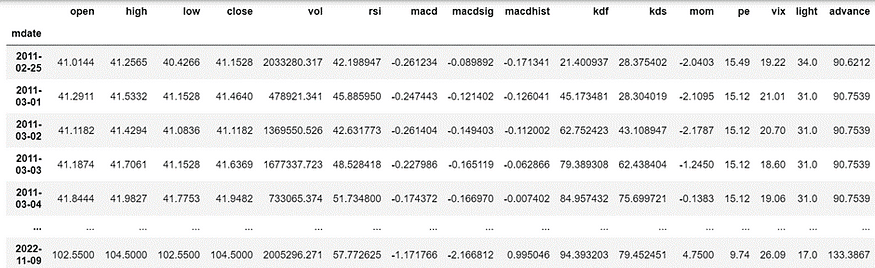
The data used includes the ex-dividend and adjusted stock prices, as well as the opening price, closing price, highest price, lowest price, and trading volume for the Taiwan 50 Index (0050) spanning from January 2011 to November 2022.
coid = "0050"
mdate = {'gte':'2011-01-01', 'lte':'2022-11-15'}
data = tejapi.get('TWN/APRCD1',
                          coid = coid,
                          mdate = {'gte':'2011-01-01', 'lte':'2022-11-15'},
                          paginate=True)


#Open high, close low, trading volume
data = data[["coid","mdate","open_adj","high_adj","low_adj","close_adj","amount"]]
data = data.rename(columns={"coid":"coid","mdate":"mdate","open_adj":"open",
                   "high_adj":"high","low_adj":"low","close_adj":"close","amount":"vol"})
Besides loading Taiwan 50 Index (0050) adjustment stock price, we also need to consider other indicators in the model, such as Technical indicators(KD、RSI、MACD、MOM) and General economic indicators (Taiwan stock average price-earnings ratio, Taiwan’s business climate countermeasure signal, leading indicators, Chicago VIX index). After eliminating some null values and impractical columns, we could organize the chart below.
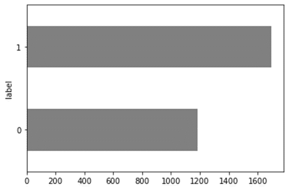
We have chosen to define trends by combining moving averages with momentum indicators. A simple criterion for identifying an upward trend is when MA10 > MA20 and RSI10 > RSI20. We labeled an upward trend as 1, otherwise it is marked as 0.
Observing the Data Distribution below, we can tell that the data distribution is not overly skewed. Due to the overall upward trend in the market, a higher number of upward trends is a regular occurrence.
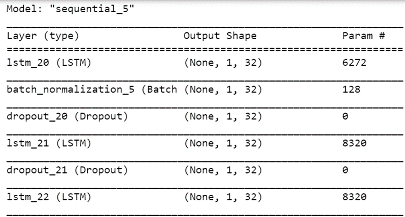
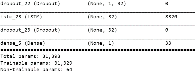
Before processing, we standardized data by cutting samples into learning and test, whose ratio is 7:3, setting the training data time range as 2011.02.25- 2019.05.08 and the test data time range as 2019.05.09- 2022.11.15. After preparing the data, we reshaped them into three Dimensions to suit the LSTM Model, which includes four layers with Dropout to prevent overfitting. Model Structures can take the figures below as references.
Boost Your Indices universe with TEJ premium Database!
Build your Quant Data feeds and Transform Insights Into Decisions.
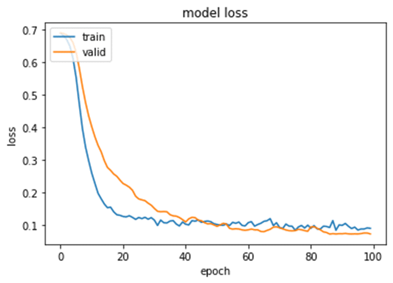
Set the number of epochs to 100. By examining the Model Loss chart, it’s evident that during the training process, the two lines converged, which indicates that the model did not overfit.
In addition, the figure below shows the importance of different feature indicators. It indicates that MACD, Taiwan Stock Average P/E Ratio, and RSI are essential features in this Model.

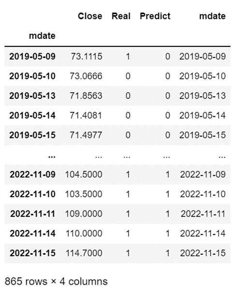
Comparing Real Labels and Model Predictions (Predictions), we found that the test set’s accuracy is as high as 95.49%, indicating that the LSTM model can effectively execute our strategy.
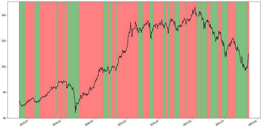
To better understand the performance, we visualize our strategy in the LSTM Strategy Trend Prediction Chart, where red represents an upward trend, and green represents a downward trend.
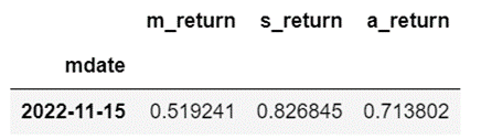
Next, we backtested the strategy. When the trend signal is upward, buy one position and hold it. On the other hand, when the trend signal turns downward, sell the original position and take a short one, holding it until the next signal as an upward trend, at which point, close the position. The cumulative return of the LSTM strategy, named ‘s_return,’ is 82.6%. The actual strategy (MA+MOM) cumulative return, ‘a_return,’ is 71.3%. The cumulative return for large-cap Buy and Hold, as ‘m_return,’ is 52%.
*Note: This strategy does not account for transaction costs; all capital is used for entering and exiting positions.
*Note: This strategy does not account for transaction costs, and all capital is used for entering and exiting positions.
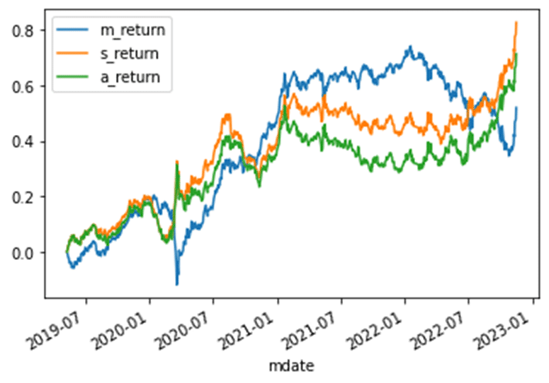
The primary purpose of this study was to examine whether LSTM could accurately identify buy and sell points according to our predefined original strategy. The result was affirmative, with a high accuracy of 95.49% and a cumulative return of 82.6% in backtesting. This performance even outperformed the original strategy and significantly beat the market’s return of 52%. We believe that one reason for outperforming the original strategy is that LSTM generated fewer trading signals during consolidation periods, avoiding the frequent whipsawing that can lead to reduced trading performance.
Lastly, we would like to reiterate that the assets mentioned in this article are for illustrative purposes only and do not constitute recommendations or advice regarding any financial products. Therefore, if readers are interested in topics such as strategy development, performance testing, empirical research, etc., you are welcome to explore the solutions available on our website, which provide comprehensive databases and tools for various analyses.
Complete Code
Further Reading
Related Link
