Using deep learning model to predict stock price?

Table of Contents
Predicting stock prices has been pursued by people, but the randomness of stock prices not easy to forecast. With the progress of data science, the calculation cost has been greatly reduced. This article use more complex deep learning model for stock prices prediction compare to [Quantitative Analysis (3)] Predict the market?! We use the opening price, the highest price, the lowest price, the closing price and the trading volume of the previous ten days to predict the closing price of next day.
This article uses Google colab as the editor
import numpy as np
import pandas as pd
import matplotlib.pyplot as pltimport tejapitejapi.ApiConfig.api_key=###yourkey##################import tensorflow as tf
from keras.layers.core import Dense, Dropout, Activation
from keras.callbacks import EarlyStopping,ModelCheckpoint
from keras.models import Sequential
from keras.layers import LSTM
from sklearn.preprocessing import MinMaxScaler
Securities trading data sheet: listed company, over-the-counter (OTC) share price(day), the database code is (TWN/EWPRCD)
Establish RMSE to evaluate the predictive ability of the model, and converting data into the form of the LSTM input as shown in the figure below:
(batch_size, time_steps, seq_len): 1163 groups, 5 days, 5 variables

Dataset: input training data
Target: forecasting data
Start_index: It’s always start at 0 because it will group itself.
End_index: destination, set 0
History_size: input length, this article chooses 10
Target_size: prediction length, this article chooses 1
def root_mean_squared_error(y_true, y_pred):
    return np.sqrt(np.mean(np.square(y_pred - y_true)###calculate Rmsedef multivariate_data(dataset, target, start_index, end_index, history_size,
                      target_size, single_step=False):
  data = []
  labels = []

  start_index = start_index + history_size
  if end_index is None:
    end_index = len(dataset) - target_size

  for i in range(start_index, end_index):
    indices = range(i-history_size, i)
    data.append(dataset[indices])

    if single_step:
      labels.append(target[i+target_size])
    else:
      labels.append(target[i:i+target_size])

  return np.array(data), np.array(labels)
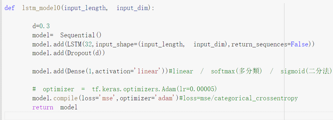
The next step is concating the model, dropout is used to prevent overfitting, this article will not explain the principle. We can adjust d between 0 to 1.
Input length is the input time length, we choose 10 days in the article.
Input_dim is the number of variables; we have 5 variables in this article.
Return_sequences: True is maintenance (batch, time_steps, seq_len), connecting the next LSTM set False will become one-dimensional.
Loss is trained by mean_squared_error, Optimizer use Adam.
def build_model(input_length, input_dim):    d=0.3
    model= Sequential()
    model.add(LSTM(128,input_shape=(input_length, input_dim),return_sequences=True))

    model.add(Dropout(d))

    model.add(LSTM(64,input_shape=(input_length, input_dim),return_sequences=False))

    model.add(Dropout(d))

    model.add(Dense(1,activation='linear'))
#linear / softmax(多分類) / sigmoid(二分法)

    model.compile(loss='mse',optimizer='adam')
    return mode1
coid='3037'
start='2016-01-01'
end='2022-5-22'
opts={'columns': ['open_d' ,'high_d','low_d','mdate', 'volume','close_d']}
tw=tejapi.get('TWN/EWPRCD',coid=coid,
                mdate={'gt':start,'lt':end},
                paginate=True,
                chinese_column_name=True,
                opts=opts
                )
tw.set_index("日期",drop=True,inplace=True)
tw.sort_index(inplace=True)
Set variables and dependent variables, the closing price is forecasting target, the others are variables.
y =tw["收盤價"]
x =tw
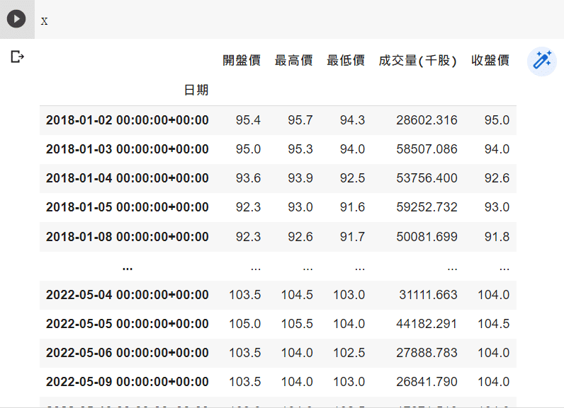
We normalize the data, which become between 0 and 1, so that the data training speed will faster and easier to converge.
scaler=MinMaxScaler(feature_range=(0,1))
y=scaler.fit_transform(y.to_frame())
scaler1=MinMaxScaler(feature_range=(0,1))
x=scaler1.fit_transform(x)
Dividing the data into training data, validation data and test data.
x,y=multivariate_data( x ,y , 0 ,None, 10 , 1 ,single_step=True)
split =0.95
x_,y_  = x[0:int(split*len(x))] , y[0:int(split*len(x))]
x_test ,y_test   = x[int(split*len(x)):] , y[int(split*len(x)):]
split= 0.8
x_train,y_train  =x_[:int(split*len(x_))] , y_[:int(split*len(x_))]
x_vaild,y_vaild  =x_[int(split*len(x_)):] , y_[int(split*len(x_)):]


The models are divided into 4 kinds, one layer is Lstm, another is Dense
my_callbacks = [
tf.keras.callbacks.EarlyStopping(patience=300, monitor ='val_loss')]

######## 在訓練組訓練,使用驗證組選取filepath="lstm.best.hdf5"checkpoint = ModelCheckpoint(filepath, monitor='val_loss', verbose=1, mode='min',save_best_only=True)call_backlist = [my_callbacks,checkpoint]lstm00 = lstm_model0(10,5)historylstm0 = lstm0.fit( x_train, y_train, batch_size=30,shuffle=False , epochs=1000,validation_data=(x_vaild,y_vaild),callbacks=call_backlist)lstm00.summary()
EarlyStopping: training parameter in training data, the lowest selection criteria is validation data. Stop training if there is no improvement after 300 epochs.
Filepath: model storage path
ModelCheckpoint: Choose the lowest val_loss as the final model
Batch: sample of each training
Epochs: frequency of training
Shuffle: True (Randomly disrupt the order), False(not disrupt the order)
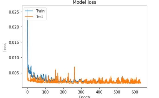
plt.plot(historylstm0.history['loss'])
plt.plot(historylstm0.history['val_loss'])
plt.title('Model loss')
plt.ylabel('Loss')
plt.xlabel('Epoch')
plt.legend(['Train', 'Test'], loc='upper left')
plt.show()
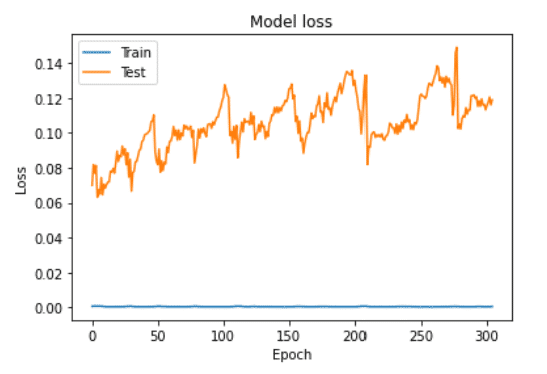
It’s found that one layer LSTM is bad, and overfitting.
lstm0train  = lstm00.predict(x_train)
lstm0val = lstm00.predict(x_vaild)
lstm0pre = lstm00.predict(x_test)pre = lstm00.predict(x_train)
pre1=lstm00.predict(x_vaild)
fc=np.concatenate((pre,pre1))
yreal=np.concatenate((y_train,y_vaild))
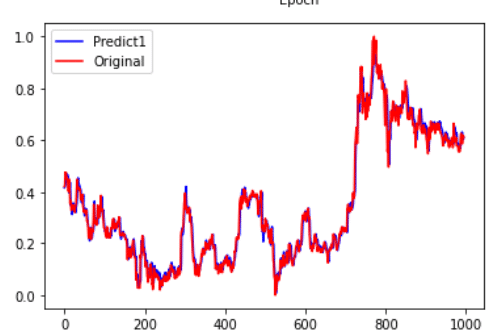
plt.figure(facecolor='white')
pd.Series(fc.reshape(-1)).plot(color='blue', label='Predict1')
pd.Series(yreal.reshape(-1)).plot(color='red', label='Original')
plt.legend()
plt.show()
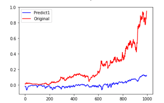
We can find that one layer LSTM model cannot grasp this time series in this picture.
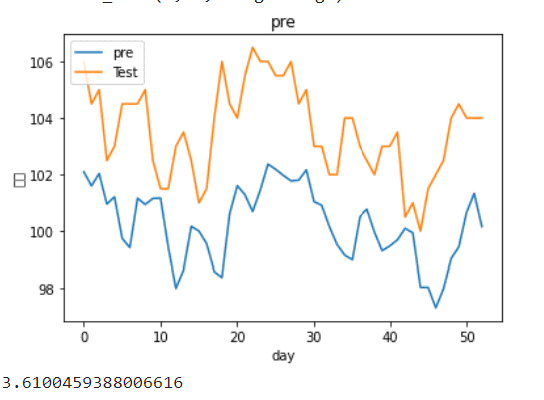
lstm0pre= scaler.inverse_transform(lstm0pre)#將資料轉換回來
y_test = scaler.inverse_transform(y_test.reshape(-1,1))plt.figure()
plt.plot(lstm0pre)
plt.plot(y_test)
plt.title('pre')
plt.ylabel('股價')
plt.xlabel('day')
plt.legend(['pre', 'Test'], loc='upper left')
plt.show()
root_mean_squared_error(lstm0pre,y_test)
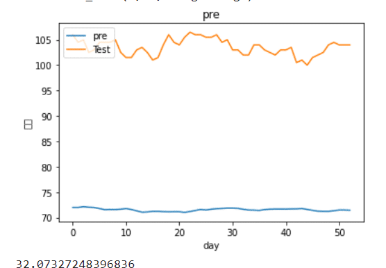
The prediction results are very bad!
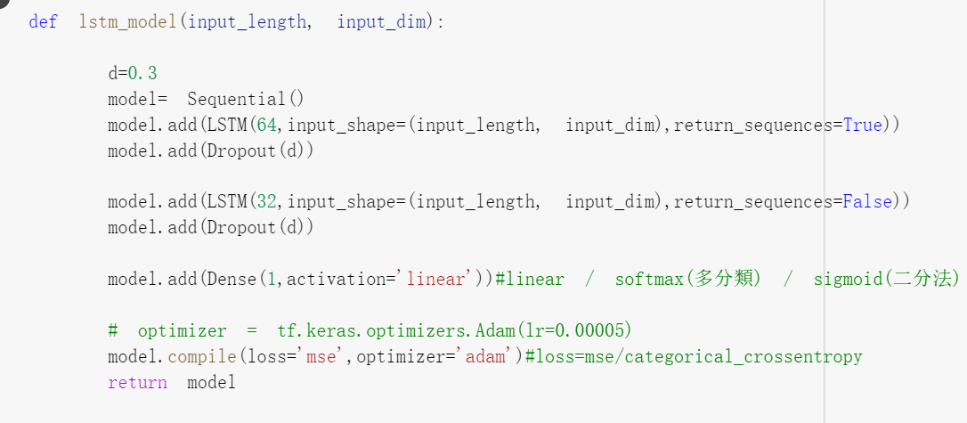
We try two layers in the next step.
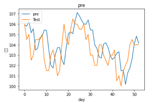
Using more complex model
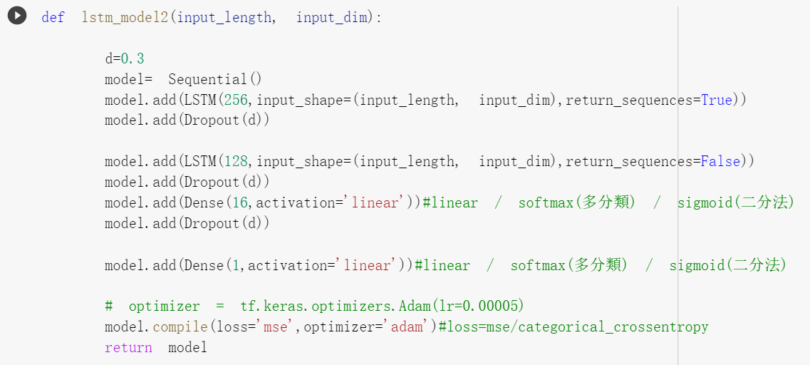
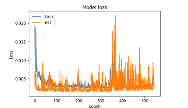
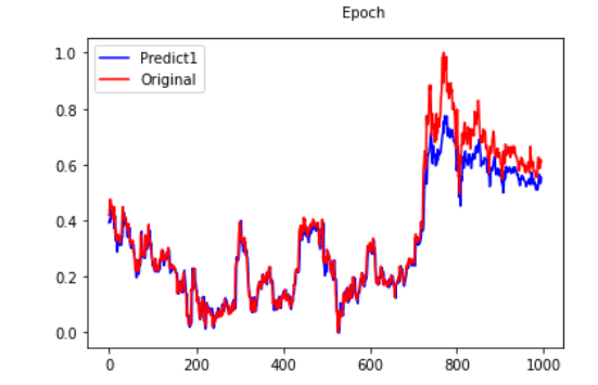
We can see that although the fitting result is good under stack-LSTM, after actual observation, it is found that the prediction of the model is only predict from yesterday to tomorrow, that is not feasible to use deep learning model to predict the next day closing price. Maybe we can change to predict the return, and add more features or stock pitching strategy to improve forecasting result. We will introduce for you later!