Table of Contents
MACD, which stands for Moving Average Convergence Divergence, is a commonly used tool in technical analysis for measuring the trend changes and momentum of an asset.
MACD consists of two main components:
The calculation steps for MACD are as follows:
MACD values can be positive, negative, or zero, and their relative positions and changes provide insights into the asset’s price trends.
Key MACD signals include:
Additionally, the MACD histogram represents the difference between the fast line and slow line, with the height of the bars indicating the magnitude of this difference.
This article uses the Mac operating system and Jupyter Notebook as the editor.
Before delving into the main content, let’s start by providing the domain and key. Following that, we will proceed with data importation. In this practical implementation, we will use TSMC (stock code: 2330) as an example, setting the time range from December 30, 2018, to May 26, 2023.
import os
import pandas as pd
import numpy as np

os.environ['TEJAPI_BASE'] = 'https://api.tej.com.tw'
os.environ['TEJAPI_KEY'] = 'your_key'
os.environ['mdate'] = '20181230 20230526'
os.environ['ticker'] = '2330'

# 使用 ingest 將股價資料導入暫存,並且命名該股票組合 (bundle) 為 tquant
!zipline ingest -b tquant

import talib
from zipline.api import order_target, record, symbol
from zipline.finance import commission, slippage
import matplotlib.pyplot as pltFirstly, let’s establish the initialize function, which is used to define the trading environment before the commencement of trading. In this example, we set:
def initialize(context):
context.sym = symbol('2330')
context.i = 0
context.invested = False
context.set_commission(commission.PerDollar(cost=0.00285))
context.set_slippage(slippage.VolumeShareSlippage())The handle_data function is used to process the daily trading strategy or actions. In this context:
We use talib to calculate the moving averages, setting the short-term window period to 12 days, the long-term window period to 26 days, and the MACD line’s window period to 9 days.
In addition to the default output information, we also want to record additional information during the execution of the trading strategy, such as the closing price, fast line index, slow line index, buy signal status, sell signal status, etc. Therefore, in the ‘record’ section, we add output fields accordingly.
def handle_data(context, data):
trailing_window = data.history(context.sym, 'price', 35, '1d')#35 = 26 + 9
if trailing_window.isnull().values.any():
return

short_ema = talib.EMA(trailing_window.values, timeperiod = 12)
long_ema = talib.EMA(trailing_window.values, timeperiod = 26)
dif = short_ema - long_ema
MACD = talib.EMA(dif, timeperiod = 9)
bar = dif - MACD
buy = False
sell = False

# Trading logic
#condition1
if (dif[-2] < MACD[-2]) and (dif[-1] > MACD[-1]) and (bar[-2] < 0) and (bar[-1] > 0):

order_target(context.sym, 1000)
context.invested = True
buy = True

#condition2
elif (dif[-2] > MACD[-2]) and (dif[-1] < MACD[-1]) and (bar[-2] > 0) and (bar[-1] < 0) and context.invested:
order_target(context.sym, 0)
context.invested = False
sell = True

# Save values for later inspection
record(TSMC = data.current(symbol('2330'), 'close'),
dif = dif[-1],
MACD = MACD[-1],
bar = bar[-1],
buy = buy,
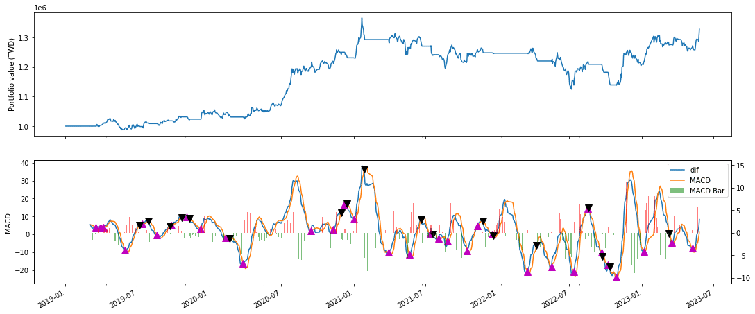
sell = sell)In the analyze function, utilize matplotlib.pyplot to draw the portfolio value line chart and MACD indicator chart. We plan to generate two charts. The first one is the portfolio value line chart, responsible for recording the trend of the portfolio value. The second one is the MACD indicator chart, tasked with documenting the trends of the fast line, slow line, MACD histogram, and marking buy and sell points.
# Note: this function can be removed if running
# this algorithm on quantopian.com
def analyze(context=None, results=None):
import matplotlib.pyplot as plt
import logbook
logbook.StderrHandler().push_application()
log = logbook.Logger('Algorithm')

fig = plt.figure()
ax1 = fig.add_subplot(211)
results.portfolio_value.plot(ax=ax1)
ax1.set_ylabel('Portfolio value (TWD)')
ax2 = fig.add_subplot(212)
ax2.set_ylabel('MACD')
# If data has been record()ed, then plot it.
# Otherwise, log the fact that no data has been recorded.
if 'dif' in results and 'MACD' in results:
results[['dif', 'MACD']].plot(ax=ax2)
ax2.plot(
results.index[results["buy"] == True],
results.loc[results["buy"] == True, 'MACD'],
'^',
markersize=10,
color='m',
)
ax2.plot(
results.index[results["sell"] == True],
results.loc[results["sell"] == True, 'MACD'],
'v',
markersize=10,
color='k',
)
ax3 = ax2.twinx()
colors = ["red" if i > 0 else "green" for i in results['bar']]
ax3.bar(results.index, results['bar'], color=colors, alpha=0.5, width=0.4, label='MACD Bar')

lines, labels = ax2.get_legend_handles_labels()
bars, bar_labels = ax3.get_legend_handles_labels()
ax2.legend(lines + bars, labels + bar_labels, loc='upper right')

plt.gcf().set_size_inches(18, 8)
else:
msg = 'TSMC - dif and MACD data not captured using record().'
ax2.annotate(msg, xy=(0.1, 0.5))
log.info(msg)
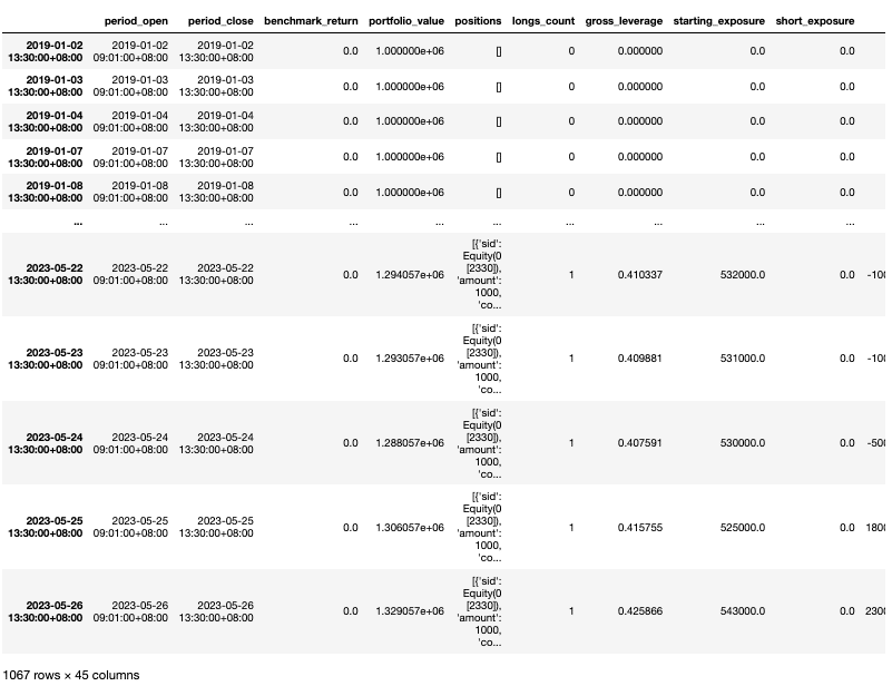
plt.show()Utilize the ‘run_algorithm’ function to execute the compiled trading strategy. Set the trading period from December 30, 2018, to May 26, 2023, with an initial capital of 100,000 CNY. Employ the ‘tquant’ dataset. The output variable ‘results’ will represent the daily performance and details of the trades.
from zipline import run_algorithm

start_date = pd.Timestamp('2018-12-30',tz='utc')
end_date = pd.Timestamp('2023-05-26',tz='utc')
results = run_algorithm(start= start_date,
end=end_date,
initialize=initialize,
capital_base=1e6,
analyze=analyze,
handle_data=handle_data,
data_frequency='daily',
bundle='tquant'
)

Based on the above report, we can observe that the portfolio value increased by approximately thirty percent. Through the MACD indicator chart, we gain a clear understanding of the timing of each trading action and trend performance. With TQuant Lab, we can significantly reduce code complexity, implementing complex backtesting systems with minimal code. However, it’s important to note that while MACD is a popular technical analysis tool, it is not absolutely reliable, and using it in isolation may generate false signals. Typically, technical analysts combine MACD with other indicators and analysis methods for more accurate judgments.
However, it is crucial to reiterate that the targets mentioned in this article are for illustrative purposes only and do not represent recommendations or advice on any financial products. Additionally, the outcomes generated by the language model do not guarantee absolute correctness and require further confirmation. Therefore, readers interested in topics such as strategy construction, performance backtesting, and research evidence are encouraged to explore solutions available in TEJ E Shop, which provides comprehensive databases for various tests.