Analyze the relationship between the company’s earnings management and the earnings-price ratio group

Table of Contents
Investors care about earnings which is one of the key indicators. future earnings trends will affect investors’ willingness to hold stocks. If investors expect an increase in the company’s earnings, they will improve their willingness to hold stocks. Earnings can be divided into cash and accruals, and accruals can be divided into discretionary and non-discretionary. Discretionary accruals is manipulated by the company’s management. According to the past research, company management has incentives to achieve its proposed earnings target by accounting principles, Discretionary power, and so on.
In the case of information asymmetry between investors and company management, company management executes earnings management by discretionary accruals. Investors may overestimate the company’s true earnings and the company’s future stock price. Measuring the company’s earnings management each year can help us avoid to hold companies with higher earnings management in the same industry.
Windows OS and Jupyter Notebook
# 功能模組
import pandas as pd
import numpy as np
import statsmodels.api as sm
import matplotlib.pyplot as plt
from scipy.stats import wilcoxon# TEJ API
import tejapi
tejapi.ApiConfig.api_key = 'Your key'
Step 1. Obtain industry code, financial data and stock price
# 匯入 台灣交易所所有代碼
code = tejapi.get("TWN/EWNPRCSTD",
                  paginate=True,
                  opts={'columns':['coid', 'mdate', 'stypenm','market','tseindnm']},
                  chinese_column_name=True)
# 匯入 財務資料
data = tejapi.get('TWN/AIM1A',
                  coid = code['證券碼'].tolist(),
                  mdate= {'gte': '2012-01-01','lte':'2020-12-31'},
                  opts={'pivot':True,
                        'columns':['coid', 'mdate','0010','0130','R531',
                                   '7210','3100','0400','3990']},
                  chinese_column_name=True,
                          paginate=True)
# 匯入 財報發布日
data_annouce = tejapi.get('TWN/AIFINA',
                          coid = code['證券碼'].tolist(),
                          mdate= {'gte': '2012-01-01','lte':'2020-12-31'},
                          opts={'columns':['coid', 'mdate', 'a0003']},
                          chinese_column_name=True,
                          paginate=True)
The stock price is the daily data. There are at least a thousand data for a stock. We can use the paginate=True parameter to obtain data, but the maximum total number of single transactions is 1,000,000. Therefore, we can group the companies into groups of 50 so that we can collect datas by for loop.
groups = []
while True:
    if len(security_list) >= 50:
        groups.append(security_list[:50])
        security_list = security_list[50:]
    elif 0 <= len(security_list) < 50:
        groups.append(security_list)
        break# 匯入未調整股價
data_price = pd.DataFrame()
for group in groups:
    data_price = data_price.append(tejapi.get('TWN/APRCD',
                                              coid = group,
                                              mdate= {'gte': '2013-03-01','lte':'2021-3-31'},
                                              opts={'columns':['coid', 'mdate','close_d']},
                                              chinese_column_name = True,
                                              paginate = True)).reset_index(drop=True)
Step 2. Keep the closing price at the end of March and the end of the year data
First, we rename column name in different dataframe so that we can avoid duplicate merge key column in merged output. Second, we only retain the stock data at the end of March each year in data_price because the denominator of the earnings-price ratio is limited to the closing price at the end of March each year. For the same reason, we only retain the year-end data in data.
# 資料前處理
code = code.rename({'證券碼': '公司'}, axis=1) # 改名字
data = data.rename({'公司代碼':'公司'}, axis=1) # 改名字
data_annouce = data_annouce.rename({'年/月':'財報年月'}, axis=1) # 改名字
data_price = data_price.rename({'證券代碼':'公司'}, axis=1) # 改名字data_price['年'] = data_price['年月日'].dt.year - 1 # 改成財報年
data_price = data_price[data_price['年月日'].dt.month == 3]
data_price = data_price.drop_duplicates(subset=['公司','年'], keep='last') # 只保留三月底收盤價data['年'] = data['財報年月'].dt.year
data = data.drop_duplicates(subset=['公司','年'], keep='last') # 只保留年底資料
Step 3. Combine data from different databases
# 合併資料
data = data.merge(code[['TSE產業名','公司']] ,how = 'left' ,on=['公司'])
data = data.merge(data_annouce,how = 'left' ,on=['公司','財報年月'])
data = data.merge(data_price[['公司','年','收盤價(元)']] ,how = 'left' ,on=['公司','年'])
We merge the financial report and the stock price data into one by company name and date.

Step 1. Prepare financial information required for DCA
We use Jones (1991) model in this article. Jones researched the part of accruals affected by the economic environment is related to sales; the gross amount of depreciable assets is related to non-discretionary depreciation expenses in total accruals. Meanwhile, we have a sort-out in the different industry business models and scale companies.
# 計算 DCA data['Total accrual'] = (data['常續性稅後淨利'] - data['來自營運之現金流量']) * data['DCA 前期資產總額倒數'] # Ydata['DCA 前期資產總額倒數'] = 1 / data.groupby('公司')['資產總額'].shift(1) # X0
data['DCA 營業收入差'] = data.groupby('公司')['營業收入淨額'].diff() * data['DCA 前期資產總額倒數'] # X1
data['DCA 不動產廠房及設備'] = data['不動產廠房及設備'] * data['DCA 前期資產總額倒數'] # X2
data['DCA 營業收入差 - 應收差'] = (data.groupby('公司')['營業收入淨額'].diff() - \
                           data.groupby('公司')['應收帳款及票據'].diff()) * data['DCA 前期資產總額倒數'] # X1
We sort firms into 14 groups based on similar industry so that we avoid too few firms in a single industry and unreliable statistics. Meanwhile, we run regression by group to reduce industry difference and use the previous period of total asset to deflate other financial factors to reduce size difference.
# 分組相似產業
data['產業分組'] = \
    np.select([(data['TSE產業名'].isin(["食品工業","紡織纖維","造紙工業"])) ,
               (data['TSE產業名'].isin(["塑膠工業","橡膠工業","化學工業","油電燃氣業"])),
               (data['TSE產業名'].isin(["汽車工業","鋼鐵工業"])),
               (data['TSE產業名'].isin(["電機機械","電器電纜"])),
               (data['TSE產業名'].isin(["水泥工業","建材營造","玻璃陶瓷"])),
               (data['TSE產業名'].isin(["資訊服務業","電子商務","貿易百貨"])),
               (data['TSE產業名'].isin(["觀光事業","航運業","文化創意業"])),
               (data['TSE產業名'].isin(["生技醫療"])),
               (data['TSE產業名'].isin(["光電業"])),
               (data['TSE產業名'].isin(["半導體"])),
               (data['TSE產業名'].isin(["電腦及週邊"])),
               (data['TSE產業名'].isin(["通信網路業"])),
               (data['TSE產業名'].isin(["電子零組件"])),
               (data['TSE產業名'].isin(["其他電子業","電子通路業","農業科技","其他"]))],
              list(range(14)), default = np.nan)

Step 2. Calculate annual DCA in different industries and firms
Total assets, operating income, and real estate plant and equipment are explanatory variables, and accruals is response variable. We get the observed accruals and the actual accruals by regression analysis. DCA is actual accruals minus observed accruals. If DCA is greater than 0, it means the company’s earnings management is greater than the company’s industry.
# 計算 DCA
def regress(data):
    '''
    每年不同產業分組跑迴歸,主要用來獲得迴歸係數
    '''
    data = data[['Total accrual','DCA 前期資產總額倒數','DCA 營業收入差','DCA 不動產廠房及設備']].dropna()
    Y = data['Total accrual']
    X = data[['DCA 前期資產總額倒數','DCA 營業收入差','DCA 不動產廠房及設備']]
    X = X.rename(columns={"DCA 前期資產總額倒數": "alpha 前期資產總額倒數",
                          "DCA 營業收入差": "alpha 營業收入差",
                          "DCA 不動產廠房及設備": "alpha 不動產廠房及設備",})
    try:
        result = sm.OLS(Y, X).fit()
        return result.params
    except ValueError:
        passdata = data.merge(data.groupby(['財報年月','產業分組']).apply(regress).reset_index(),
                        how = 'left' ,on = ['財報年月','產業分組'])data['Normal accrual'] = (data['alpha 前期資產總額倒數'] * data['DCA 前期資產總額倒數'] \
                          + data['alpha 營業收入差'] * data['DCA 營業收入差 - 應收差'] \
                              + data['alpha 不動產廠房及設備'] * data['DCA 不動產廠房及設備'])data['DCA'] = data['Total accrual'] - data['Normal accrual']
Step 3. Profit-to-cost ratio grouping
We sort firms into groups based on earnings-price ratio to analyze the specified group whether there are a significant abnormality DCA. That is, there are a significant abnormality earnings management in the specified group.
# 計算益本比,並以0.0125分組。
def cal_EP_label():
    '''獲得 EP ratio分組下的公司數,num=33,切0.025'''
    label = np.linspace(-0.2, 0.2, num=33).tolist()
    label = [ '%.4f' % elem for elem in label ]
    label.insert(0,-np.inf)
    label.insert(len(label),np.inf)
    label = np.array(label, dtype=float)
    return labeldata['益本比'] = data['每股盈餘'] / data['收盤價(元)']
data['益本比分組'] = pd.cut(data['益本比'],bins = cal_EP_label() ,right=True)

Step 1. Create a graph to analyze the distribution of earnings-price ratio
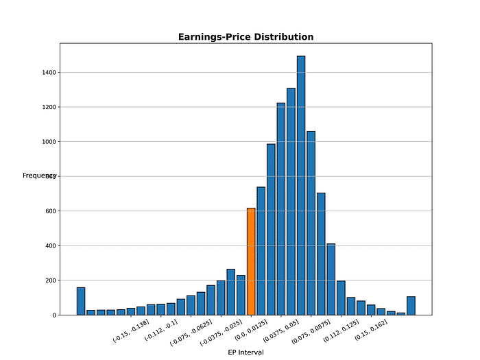
In the figure below, there is a significant difference between the number of companies whose earnings-price ratio distribution is in (-0.0125, 0.0) and (0.0, 0.0125]. Does this indicate that the company’s management have loss aversion when they face with earnings losses? Therefore, the company’s management is unwilling to explain the losses to the shareholders and they have an incentive to manipulate the EPS from negative to positive.
#%% 做圖 觀察益本比分組狀況fig = plt.figure(figsize = (12,9))
ax = fig.add_subplot()factor = data.groupby(['益本比分組'])['公司'].count().reset_index()['益本比分組'].astype(str)
value = data.groupby(['益本比分組'])['公司'].count().reset_index()['公司']
ax.bar(factor,value,fill = '#eb3434',edgecolor = 'black')
ax.bar('(0.0, 0.0125]',value[17],fill = '#eb344f',edgecolor = 'black')
ax.set_title('Earnings-Price Distribution',
             fontsize=16,
             fontweight='bold')
ax.set_xticks(['(-0.15, -0.138]','(-0.112, -0.1]','(-0.075, -0.0625]','(-0.0375, -0.025]','(0.0, 0.0125]',
              '(0.0375, 0.05]','(0.075, 0.0875]','(0.112, 0.125]','(0.15, 0.162]'])
plt.grid(axis='y')
plt.xticks(rotation=30)
plt.xlabel('EP Interval',fontsize=12)
plt.ylabel('Frequency',fontsize=12, rotation=0)
plt.show()

Step 2. Make a table to observe the relationship between the earnings-price ratio groups and the degree of earnings management
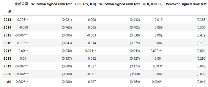
The median test of Wilcoxon signed-rank test is performed on the earnings-price ratio groups, and it was found that the median of DCA of all companies is -0.002 being significantly different from 0. However, the company’s earnings-price ratio is in (-0.0125, 0.0) and (0.0, 0.0125), the median DCA is 0.004 being significantly different from 0. It can be seen that the compnay’s earnings-price ratio is in (0.0, 0.0125). the companys with earnings management is widespread.
def cal_wilcoxon(group):
    return pd.DataFrame({'DCA': group.median(),
                         'p-value': wilcoxon(group)[1]}, index = [0])def add_star(df,p_value):
    '''
    p-values of the Wilcoxon signed rank test <= 0.01,則係數新增***
    0.01 < p-values of the Wilcoxon signed rank test <= 0.05,則係數新增**
    0.1 < p-values of the Wilcoxon signed rank test <= 0.01,則係數新增*
    '''
    df = np.select([(p_value <= 0.01),
                      (p_value > 0.01) & (p_value <= 0.05),
                      (p_value > 0.05) & (p_value <= 0.1)],
                     [df.apply(lambda x: '%.3f'%x + '***'),
                      df.apply(lambda x: '%.3f'%x + '**'),
                      df.apply(lambda x: '%.3f'%x + '*')],
                     default = df.apply(lambda x: '%.3f'%x))
    return dfdef run_data_cal_wilcoxon(df):
    '''p-values of the Wilcoxon signed rank test for one sample median DCA equal to 0'''
    finaldf = pd.DataFrame()

    for data in df:

        temp = data.dropna(subset=['DCA']).groupby('年')['DCA'].\
            apply(cal_wilcoxon).reset_index(level=1, drop=True)

        temp.loc['All','DCA'] = data.dropna(subset=['DCA'])['DCA'].median()
        temp.loc['All','p-value'] = wilcoxon(data.dropna(subset=['DCA'])['DCA'])[1]

        temp['DCA'] = add_star(temp['DCA'],temp['p-value'])
        temp['p-value'] = temp['p-value'].apply(lambda x: '(' + '%.3f'%x + ')')

        finaldf = pd.concat([finaldf, temp], axis=1)

    return finaldfTable = run_data_cal_wilcoxon([data,
                               data[data['益本比分組'].astype(str).isin(['(-0.025, 0.0]'])],
                               data[data['益本比分組'].astype(str).isin(['(0.0, 0.025]'])]])

「Losses loom larger than gains」 meaning that people by nature are aversive to losses. Therefore, when a company’s management faces a small loss, there is a very high incentive to manipulate earnings management through Discretionary Accruals. they can change EPS from negative to positive to fit the expectations of shareholders and investors in the capital market.
In this paper, we can identify which companies’ DCA being significantly higher than the industry average DCA and check whether the company’s earnings-price ratio is in the range of (-0.0125, 0.0) and (0.0, 0.0125). If company’s earnings-price ratio is in the range of (-0.0125, 0.0) and (0.0, 0.0125) and DCA is higher than 0, the company most likely have an earnings management.