Optimizing investment portfolios using PCA (Principal Component Analysis)

Table of Contents
Article Difficulty:★★★★☆
The essence of mathematics is not to complicate simple things but to simplify complex things.” – Stan Gudder
Principal Component Analysis (PCA), a crucial technique in unsupervised learning, is widely used in the fields of machine learning and statistics to analyze data and reduce data dimensionality. Its core idea is to break down the original data into representative principal components, achieving dimensionality reduction and providing a new description of the data.
The main purpose of this study is to utilize daily stock return data, apply PCA to obtain principal components, and construct an investment portfolio. Readers of this article will see the following key points:
This article uses Windows OS and employs Jupyter as the editor.
import tejapi
import pandas as pd
import numpy as np
import matplotlib.pyplot as plt
import seaborn as sns
from sklearn.preprocessing import StandardScaler
from sklearn.decomposition import PCA

tejapi.ApiConfig.api_key = "Your Key"
0050 Index Constituent Data Set — Listed OTC Index (TWN/EWISAMPLE)
0050 Stock price return (day) – rate of return (TWN/APRCD2)
0050 Adjustment of stock price (day) — ex-dividend adjustment (TWN/APRCD1)
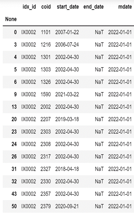
Loading Index Data Period: 2013.01.01–2022.11.24 Loading 0050 Constituent Stocks with filtering based on the “end_date” column to select stocks that are currently part of the constituents.
mdate = {'gte':'2000-01-01', 'lte':'2022-11-24'}
data = tejapi.get('TWN/EWISAMPLE',
                  idx_id = "IX0002",
                  start_date = mdate,
                          paginate=True)

data1 = data[data["end_date"] < "2022-11-24"]
diff_data = pd.concat([data,data1,data1]).drop_duplicates(keep=False)
coid = list(diff_data["coid"])
print(len(coid))
diff_data
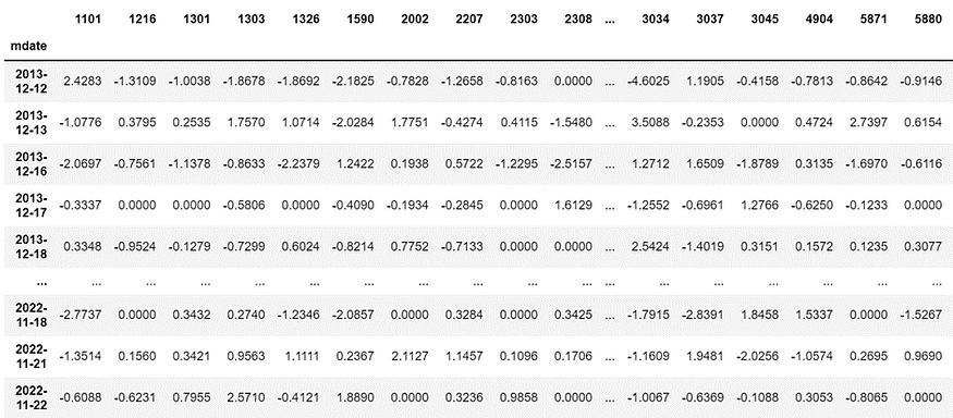
0050 Loading Returns Data
for i in range(0,len(coid)):
    print(i)
    if i == 0:
        df = tejapi.get('TWN/EWPRCD2',
                                  coid = coid[i],
                                  mdate = {'gte':'2013-01-01', 'lte':'2022-11-24'},
                                  paginate=True)
        df.set_index(df["mdate"],inplace=True)
        Df = pd.DataFrame({coid[i]:df["roia"]})
    else:
        df = tejapi.get('TWN/EWPRCD2',
                                  coid = coid[i],
                                  mdate = {'gte':'2013-01-01', 'lte':'2022-11-24'},
                                  paginate=True)
        df.set_index(df["mdate"],inplace=True)
        Df1 = pd.DataFrame({coid[i]:df["roia"]})
        Df = pd.merge(Df,Df1[coid[i]],how='left', left_index=True, right_index=True)
The return rate information of ASE Investment Holdings (3711) was only available after 2018/04/30 and was deleted.
Shanghai Commercial Savings Bank ( 5876 ) was listed after 2014/09/25 and only had rate of return information, so it was excluded.
Silicon Power-KY (6415) was listed after 2013–12–12, and the rate of return data is excluded.
del Df["3711"]
del Df["5876"]
del Df["6415"]
Therefore, this article focuses on the 47 constituent stocks of the Taiwan 0050 Index up to 2022/11/24, excluding the three stocks mentioned above.
First, we need to have a basic understanding of the dataset. By observing the correlations between the returns of each constituent stock, we can see a significant positive correlation among daily returns. Therefore, the data can be represented in a lower dimension, which is less than the current 47 dimensions.
cor = Df.corr()
plt.figure(figsize=(30,30))
plt.title("Correlation Matrix")
sns.heatmap(cor, vmax=1,square=True,annot=True,cmap="cubehelix")

Before building the model, we do not know the importance of each feature in the dataset, which can lead to a significant loss of information. Therefore, standardizing each feature to have the same range of values is necessary, followed by applying PCA.
scale = StandardScaler().fit(Df)
rescale = pd.DataFrame(scale.fit_transform(Df),columns=Df.columns,index=Df.index)
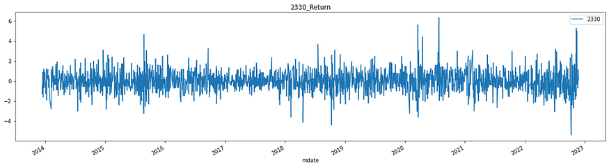
#標準化視覺化
plt.figure(figsize=(20,5))
plt.title("2330_Return")
rescale["2330"].plot()
plt.grid=True
plt.legend()
plt.show()
Model Setup
We aim to reduce the original 47-dimensional data to 10 dimensions, representing the original data using 10 principal components.
n_components = 10
pca = PCA(n_components=n_components)
Pc = pca.fit(X_train)
PCA Explaining Variables
The first principal component represents the largest variance in the original data, the second principal component represents the second-largest variance, and so on in descending order of variance.
fig, axes = plt.subplots(ncols=2)
Series1 = pd.Series(Pc.explained_variance_ratio_[:n_components ]).sort_values()
Series2 = pd.Series(Pc.explained_variance_ratio_[:n_components ]).cumsum()

Series1.plot.barh(title="Explained Variance",ax=axes[0])
Series2.plot(ylim=(0,1),ax=axes[1],title="Cumulative Explained Variance")
print("變數累積解釋比例:")
print(Series2[len(Series2)-1:len(Series2)].values[0])
print("各變數解釋比例:")
print(Series1.sort_values(ascending=False))
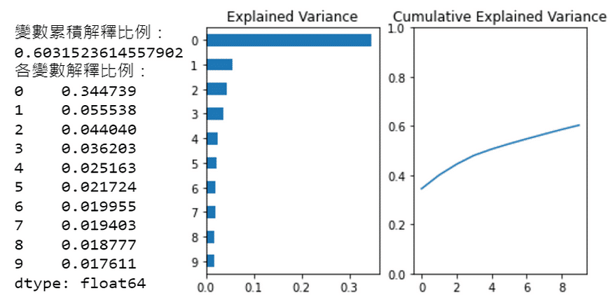
From the left chart, it can be seen that the first 10 principal components explain the variance. The first principal component alone accounts for 35% of the variance in the original data, which means it explains 35% of the daily return variations in the 47 constituent stocks. This dominant principal component is often referred to as the “market” factor.
From the right chart, it can be observed that the first 10 principal components collectively explain approximately 60% of the variance in the daily returns of these 47 stocks.
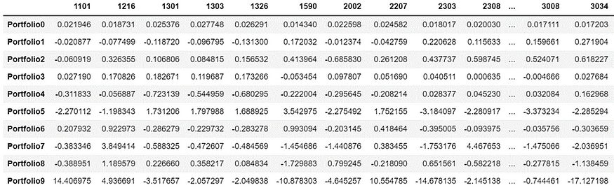
Setting Portfolio Weights
In the previous step, we examined the explained variance by the principal components. Next, we will explore the correlation of the original data, which consists of 47 stocks, with these 10 principal components. We will use this information to design the portfolio weights.
n_components = 10
weights = pd.DataFrame()
for i in range(n_components):
    weights["weights_{}".format(i)] = pca.components_[i] / sum(pca.components_[i])
weights = weights.values.T
weight_port = pd.DataFrame(weights,columns=Df.columns)
weight_port.index = [f'Portfolio{i}' for i in range(weight_port.shape[0])]
weight_port
Explaining the Portfolio Weighting Method
The first principal component explains 35% of the variance. Let’s examine the correlation of each variable (47 constituent stocks) with the first principal component.
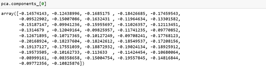
As seen from the array, the correlation of all 47 constituent stocks with the first principal component is in the same direction (all negative), and the differences in magnitude are not significant. This further validates our previous explanation that the first principal component represents the “market” factor.
weight_port.iloc[0].T.sort_values(ascending=False).plot.bar(subplots=True,figsize=(20,5),
                          legend=False,sharey=True,ylim=(-0.75,0.75))
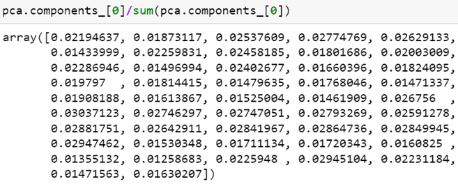
Next, we calculate the portfolio weights by taking the correlation of each stock divided by the sum of correlations of all stocks.
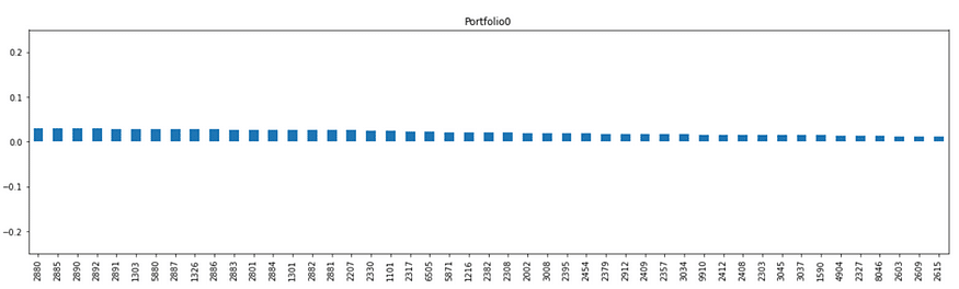
Plotting the Weights of the Top Five Principal Components in the Portfolio
weight_port[:5].T.plot.bar(subplots=True,layout = (int(5),1),figsize=(20,25),
                      legend=False,sharey=True,ylim=(-2,2))
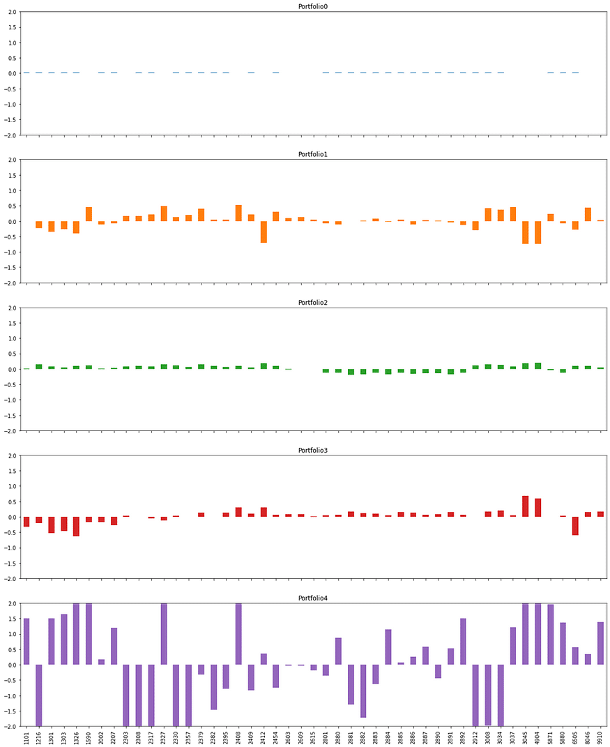
Examining the Classification Logic of Other Principal Components
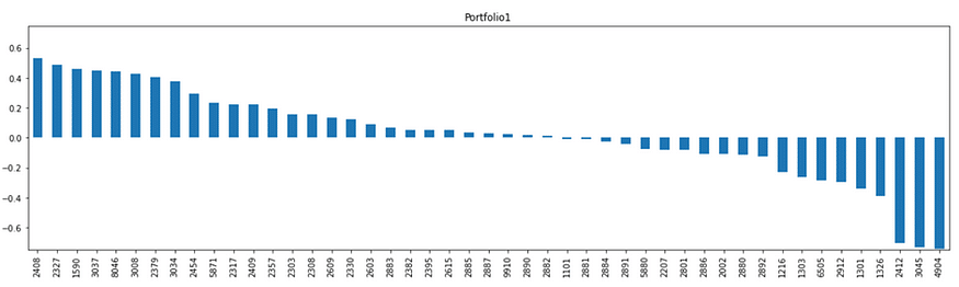
Portfolio 1
The top three are Nanya Branch (2408), Yageo (2327), and Airtec KY (1590); the last three are Far EasTone (4904), Taiwan University (3045), and Chunghwa Electronics (2412). Out of Portfolio 1, the weighting of electronic stocks is higher, while the weighting of transmission and telecommunications stocks is lower.
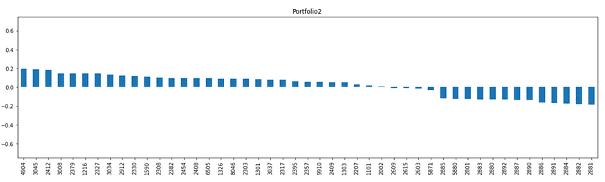
Portfolio 2
The top three stocks in Portfolio 2 are actually the three major telecommunications companies, while the later stocks are mostly from the financial sector. This suggests that Portfolio 2 is a non-financial investment portfolio.
We are using the Sharpe Ratio as our metric, which is a crucial indicator for measuring the performance and stability of an investment portfolio in fund investment or asset allocation. It represents “how much return can be obtained while enduring 1% of risk?”
In this article, the Sharpe Ratio is calculated as follows:
Sharpe Ratio = Annualized Return / Annualized Risk
def sharpe_ratio(ts_returns):
    ts_returns = ts_returns
    days = ts_returns.shape[0]
    n_years = days/252
    if ts_returns.cumsum()[-1] < 0:
        annualized_return = (np.power(1+abs(ts_returns.cumsum()[-1])*0.01,1/n_years)-1)*(-1)
    else:
        annualized_return = np.power(1+abs(ts_returns.cumsum()[-1])*0.01,1/n_years)-1
    annualized_vol = (ts_returns*0.01).std()*np.sqrt(252)
    annualized_sharpe = annualized_return / annualized_vol

    return annualized_return,annualized_vol,annualized_sharpe
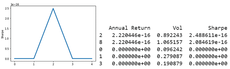
選出Top5 Portfolio
n_components = 10
annualized_ret = np.array([0.]*n_components)
sharpe_metric = np.array([0.]*n_components)
annualized_vol = np.array([0.]*n_components)
coids = X_train.columns.values
n_coids = len(coids)

pca = PCA(n_components=n_components)
Pc = pca.fit(X_train)
pcs = pca.components_
for i in range(n_components):
    pc_w = pcs[i] / sum(pcs[i])
    eigen_port = pd.DataFrame(data={"weights":pc_w.squeeze()},index=coids)
    eigen_port.sort_values(by=["weights"],ascending=False,inplace=True)
    #The daily portfolio return is obtained by taking the dot product of the portfolio weights and the daily returns of each constituent stock.
    eigen_port_returns = np.dot(X_train.loc[:,eigen_port.index],eigen_port["weights"])
    eigen_port_returns = pd.Series(eigen_port_returns.squeeze(),
                                   index = X_train.index)

    ar,vol,sharpe = sharpe_ratio(eigen_port_returns)

    annualized_ret[i] = ar
    annualized_vol[i] = vol
    sharpe_metric[i] = sharpe

sharpe_metric = np.nan_to_num(sharpe_metric)

N=5
result = pd.DataFrame({"Annual Return":annualized_ret,"Vol":annualized_vol,"Sharpe":sharpe_metric})
result.dropna(inplace=True)
#Sharpe Ratio of PCA portfolio
ax = result[:N]["Sharpe"].plot(linewidth=3,xticks=range(0,N,1))
ax.set_ylabel("Sharpe")
result.sort_values(by=["Sharpe"],ascending=False,inplace=True)
print(result[:N])
Drawing a Trend Chart of Portfolio Returns Over the Investment Period
def Backtest(i,data):
    pca = PCA()
    Pc = pca.fit(data)
    pcs = pca.components_
    pc_w = pcs[i] / sum(pcs[i])
    eigen_port = pd.DataFrame(data={"weights":pc_w.squeeze()},index=coids)
    eigen_port.sort_values(by=["weights"],ascending=False,inplace=True)
    #權重與每天報酬取內積得出每日投資組合報酬
    eigen_port_returns = np.dot(data.loc[:,eigen_port.index],eigen_port["weights"])
    eigen_port_returns = pd.Series(eigen_port_returns.squeeze(),
                                   index = data.index)

    ar,vol,sharpe = sharpe_ratio(eigen_port_returns)
    return eigen_port_returns,ar,vol,sharpe
Visualizing the Trend of Portfolio Returns
def Weight_plot(i):
    top_port = weight_port.iloc[[i]].T
    port_name = top_port.columns.values.tolist()
    top_port.sort_values(by=port_name,ascending=False,inplace=True)
    ax = top_port.plot(title = port_name[0],xticks=range(0,len(coids),1),
                  figsize=(15,6),
                  rot=45,linewidth=3)
    ax.set_ylabel("Portfolio Weight")
portfolio = 0
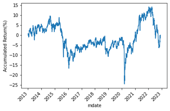
train_returns,train_ar,train_vol,train_sharpe = Backtest(portfolio,X_train)
ax = train_returns.cumsum().plot(rot=45)
ax.set_ylabel("Accumulated Return(%)")
Weight_plot(portfolio)
Summary
The provided backtesting method for the portfolio constructed using PCA shows that its performance is not favorable. This outcome was somewhat expected since PCA is primarily used for portfolio classification based on return correlations and does not guarantee good returns on its own.
This article provided an analysis of the Taiwan 50 Index (with three stocks excluded due to data availability) using PCA. It reduced the original 47 stocks to 10 principal components and constructed portfolio weights based on the correlation between the principal components and individual stocks. The article discussed each principal component, highlighting the presence of the dominant “market” factor and the logical classification ability of PCA. However, providing a detailed interpretation of the meaning of each principal component can be challenging.
In conclusion, it’s important to reiterate that the assets mentioned in this article are for illustrative purposes only and do not constitute any recommendations or advice on financial products. Therefore, readers interested in strategy development, performance testing, empirical research, and related topics are welcome to explore solutions available in the TEJ E Shop, which offers comprehensive databases for conducting various analyses and tests.
