
Table of Contents
Value at risk, VaR, means the maximum loss of a portfolio by determined confidence level and data of specific period.
The procedure of calculation is as follow:
During computing, we should notice every parameter setting and distribution of stock return so as to reflect market’s volatility on the numbers. Subsequently, we would carefully implement the process and illustrate the defect of variance-covariance method.
VaR terms applied in this article:
2. Relative VaR:The VaR compared to average return of portfolio.
(|-α| * σ) * portfolio value
3. Absolute VaR:The VaR compared to 0.
(|-α| * σ — mean) * portfolio value
Above α is the critical value of normal distribution. We would apply the the most restrict standard, 99% confidence level and Z-value equal to 2.33 to compute.
MacOS & Jupyter Notebook
#基本套件import numpy as npimport pandas as pd#繪圖套件import matplotlib.pyplot as plt%matplotlib inlineimport seaborn as snssns.set()#TEJAPIimport tejapitejapi.ApiConfig.api_key = 'Your Key'tejapi.ApiConfig.ignoretz = True
Step 1. Stock Price
The portfolio would consist of traditional , high-tech, finance and shipping corporation. We would calculate VaR and display the distribution of every stock. By combining above parts, we would make you understand the pro-and-con of Variance-Covariance VaR.
ticker = ['1476', '2330', '2882', '2603']# 儒鴻, 台積電, 國泰金, 長榮df = tejapi.get('TWN/EWPRCD', # 公司交易資料-已調整股價(收盤價)coid = ticker,mdate = {'gte':'20200101', 'lte':'20220225'},opts = {'columns': ['coid', 'mdate', 'close_adj']},chinese_column_name = True,paginate = True)df = df.set_index('日期')
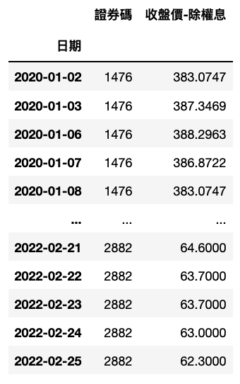
data = {}for i in ticker:p = df[df['證券代碼'] == i]p = p['收盤價(元)']data.setdefault(i, p)data = pd.concat(data, axis = 1)
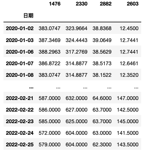
Step 3. Daily Return
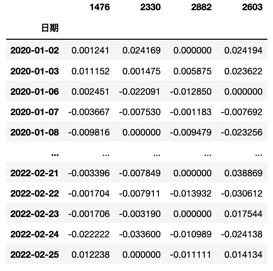
Apply Security Return Data Table to ensure the source quality. Pre-processing of return data is the same as that of price.
ret = tejapi.get('TWN/EWPRCD2',coid = ticker,mdate = {'gte':'20200101', 'lte':'20220225'},opts = {'columns': ['coid', 'mdate', 'roia']},chinese_column_name = True,paginate = True)ret = ret.set_index('日期')data2 = {}for i in ticker:r = ret[ret['證券碼'] == i]r = r['日報酬率(%)']data2.setdefault(i, r)data2 = pd.concat(data2, axis = 1)data2 = data2 * 0.01 #還原報酬率為百分之一單位基準
Step 1. Declare Empty Lists
value = data.iloc[-1] * 1000Mean = []STD = []MAX = []Min = []abs_var = []re_var = []
Firstly, we would calculate value of stocks in portfolio, assuming hold at least 1,000 share, which is the base unit in TAIEX. Subsequently, declare empty lists.
Step 2. Calculate DEAR, one-day VaR
for i in ticker:v = data2[i].std() # Standard Errormean = data2[i].mean() # Meanmaximum = data2[i].max() # Maximumminimum = data2[i].min() # Minimum# Calculate 99% Absolute VaRvar_99_ab = (abs(-2.33)*v - mean) * value[i]# Calculate 99% Relative VaRvar_99_re = (abs(-2.33)*v) * value[i]# Append those values in listsMean.append(mean)STD.append(v)MAX.append(maximum)Min.append(minimum)abs_var.append(var_99_ab)re_var.append(var_99_re)
In the loop, we firstly calculate std, mean, maximum and minimum. Secondly, compute absolute and relative VaR. Lastly, return values to empty lists.
We apply abs() during calculation of VaR, which is for the remind of that VaR concerns the downside, namely the negative, so -2.33 is adequate. However, using positive number is the convention of presenting VaR; therefore, convert -2.33 to positive by abs().
Step 3. Construct new Table
dear = pd.DataFrame({'Mean': Mean, 'STD': STD, 'Maximum': MAX, 'Minimum': Min, '99%絕對VaR': abs_var, '99%相對VaR': re_var},index = ticker)# 直接將DEAR命名為絕對、相對VaR,供後續計算使用

rho = data2.corr() # Apply ret to avoid spurious regression result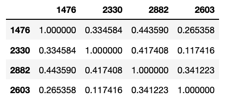
Instead of price data, we apply return data to get the correlation coefficient among stocks. By doing so, we would avoid Spurious Regression and compute correct coefficient.
Step 1. Concatenate Tables
# 將不需用到的資料剔除。dear = dear.drop(columns = ['Mean', 'STD', 'Maximum', 'Minimum'])# 合併 dear 與 rhoportfolio = pd.concat([dear, rho,], axis = 1)portfolio[['99%絕對VaR', '99%相對VaR']] = portfolio[['99%絕對VaR', '99%相對VaR']]

Step 2. Calculate VaR
part1 is the proportion of VaR of stocks itself in portfolio. As for part2, it is the VaR with the adjustment of correlation coefficient among different stocks.
part1 = sum(portfolio['99%絕對VaR']**2)part2 =2*portfolio.iat[0,3] * portfolio.iat[0,0] * portfolio.iat[1,0]+ 2*portfolio.iat[0,4] * portfolio.iat[0,0] * portfolio.iat[2,0]+ 2*portfolio.iat[0,5] * portfolio.iat[0,0] * portfolio.iat[3,0]+ 2*portfolio.iat[1,4] * portfolio.iat[1,0] * portfolio.iat[2,0]+ 2*portfolio.iat[1,5] * portfolio.iat[1,0] * portfolio.iat[3,0]+ 2*portfolio.iat[2,5] * portfolio.iat[2,0] * portfolio.iat[3,0]
Absolute VaR at 99% confidence level is 50647.78.
part1 = sum(portfolio['99%相對VaR']**2)part2 =2*portfolio.iat[0,3] * portfolio.iat[0,1] * portfolio.iat[1,1]+ 2*portfolio.iat[0,4] * portfolio.iat[0,1] * portfolio.iat[2,1]+ 2*portfolio.iat[0,5] * portfolio.iat[0,1] * portfolio.iat[3,1]+ 2*portfolio.iat[1,4] * portfolio.iat[1,1] * portfolio.iat[2,1]+ 2*portfolio.iat[1,5] * portfolio.iat[1,1] * portfolio.iat[3,1]+ 2*portfolio.iat[2,5] * portfolio.iat[2,1] * portfolio.iat[3,1]
Relative VaR at 99% confidence level is 52205.86.
According to above calculation, we conclude that maximum loss of the portfolio in one day would not exceed 52 thousands at 99 percent chance. However, market always fluctuates. Hence, keeping the calculation of VaR regularly would make our judgement more accurately.
We would display distributions of stocks so as to check severity of fat-tail.
plt.rcParams['font.sans-serif'] = ['Arial Unicode MS']fig, ax =plt.subplots(figsize = (18, 12), nrows = 2, ncols = 2)data2['1476'].plot.hist(ax=ax[0][0], bins = 100,range=(data2['1476'].min(), data2['1476'].max()), label = '儒鴻')ax[0][0].legend(loc = 2, fontsize = 30)data2['2330'].plot.hist(ax=ax[0][1], bins = 100,range=(data2['2330'].min(), data2['2330'].max()), label = '台積電')ax[0][1].legend(loc = 2, fontsize = 30)data2['2882'].plot.hist(ax=ax[1][0], bins = 100,range=(data2['2882'].min(), data2['2882'].max()), label = '國泰金')ax[1][0].legend(loc = 2, fontsize = 30)data2['2603'].plot.hist(ax=ax[1][1], bins = 100,range=(data2['2603'].min(), data2['2603'].max()), label = '長榮')ax[1][1].legend(loc = 2, fontsize = 30)plt.tight_layout()
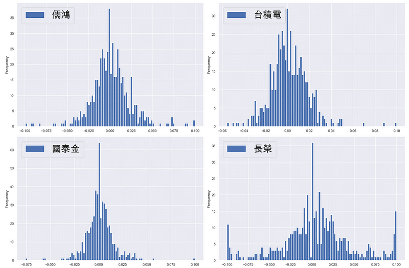
Based on above charts, it is clear that EVERGREEN’s fat-tail is the most apparent. TSMC and Eclat Textile have fat-tail but not that dramatic. As for Cathay Financial Holdings, there is almost no fat-tail.
With the process of calculation and analysis in this article, believe you would understand the procedure of Variance-Covariance Method. Firstly, calculate DEAR. Subsequently, get the correlation coefficient. Lastly, compute VaR of the whole portfolio. It is for sure that there is some disadvantages of this method and you can understand that fat-tail problem exists in these stocks. As a result, if you are curious about the solution for fat-tail, pleaser keep tracking this platform. We, later, will post new article to demonstate. In the end, welcome to purchase the plans offered in TEJ E Shop to conduct VaR calculation for your own portfolio.