
Table of Contents
Machine learning(ML), deep learning(DL), and artificial intelligence have been widely used by industries recently. Applications such as image recognition and voice recognition are common in our life.
However, wall street, the world center of finance has already recruited many statistics, mathematics even physics experts as algorithmic engineers and quantitative traders to exploit trading strategies. There had many cross-domain integrations in the finance field, and one of the most famous is the option pricing model, Black-Scholes Model(BS model). It uses the Brownian motion, which is the physic term to describe the random fluctuations in a particle’s position inside a fluid domain to quantify the daily price movement of options. Although there had some flaw in the model’s assumption, it still got the honor of the Nobel prize in economics at that time. In this case, we could know the contribution of the BS model to both academies and practices.
In this article, we would guide you to the world of machine learning, and introduce how to use it to predict market movement~
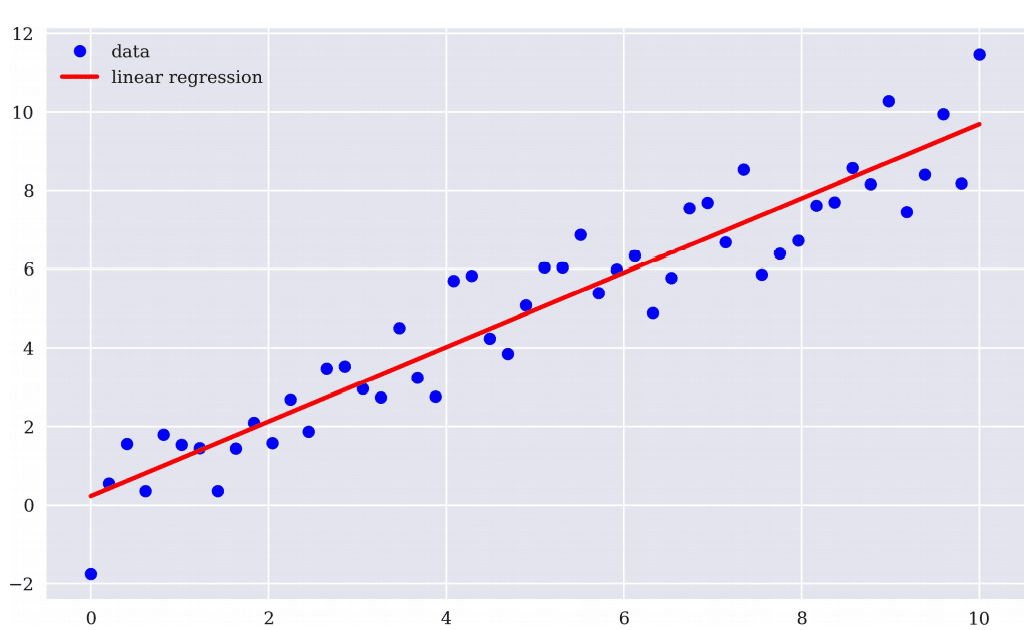
Linear regression is the statistical method to find the pattern of the data and further draw a line to fit the data. While using linear regression, we only need to determine the independent variables (X value) and dependent variables (Y value). More intuitively, for example, if we want to use today’s return to predict the future return, to meet this purpose, we take the yesterday return as the independent variable(X), the tomorrow return as dependent variables (Y).

We can find the best line to fit the data according to the formula above. The score measures by the average distance among points to the straight, called mean square error. The linear regression aims to find the best combination of the coefficients (β0, β1) that minimize the mean square error.
import pandas as pd
import numpy as np
import matplotlib.pyplot as plt
plt.style.use('seaborn')
plt.rcParams['font.sans-serif'] = ['Microsoft JhengHei']
import tejapi
tejapi.ApiConfig.api_key = 'your key'
tejapi.ApiConfig.ignoretz = TrueGrabbing the daily stock price and return of MEDIATEK (2454), the data sourced from TEJ API. In this episode, we use the securities trading database and securities return database to get the close-adjusted price and daily return.
data = tejapi.get('TWN/EWPRCD',
                  coid='2454',
                  paginate = True,
                  chinese_column_name = True
                 )
return_ = tejapi.get('TWN/EWPRCD2',
                  coid='2454',
                  paginate = True,
                  chinese_column_name = True
                 )
data['報酬率%'] = return_['日報酬率(%)']Grabbing the daily stock price and return of MEDIATEK (2454), the data sourced from TEJ API. To get the close-adjusted price and daily return, we extract the data from the securities trading table and the securities return table. (Data source)
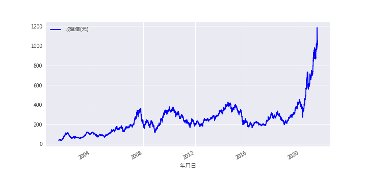
The figure below shows that stock prices grow along with time. In other words, the overall trend of the stock price is upward, and we can also say stock price is non-stationary data. So, if we use yesterday’s stock price as X, today’s stock price as Y.
Even though the statistic result is significant, but just a coincidence. There doesn’t have a strong relation between X and Y. This kind of circumstance so-called spurious regression. (reference)
⏰ The solution to fix non-stationary data:
The first-order difference means to calculate the stock return. After calculation, the trend of the data has been removed. Now, we can put the data into the linear regression model.
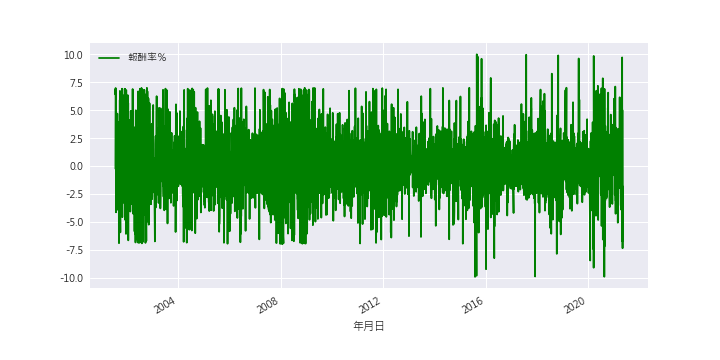
According to the graph below, we realize that it’s hard to predict return by linear regression model.
# 用昨天(第t-1日)的報酬率去預測今天(第t日)的報酬率
# 因前兩個位置的值為NA,故取第3個位置以後的數值
x = data['報酬率%'].shift(1)[2:].values
y = data['報酬率%'][2:].values
reg = np.polyfit(x,y,deg=1)
# 繪圖
plt.figure(figsize=(10,6))
plt.plot(x, y, 'bo', label='data')
plt.plot(x, np.polyval(reg,x),'r',label='linear regression')
plt.legend(loc=0)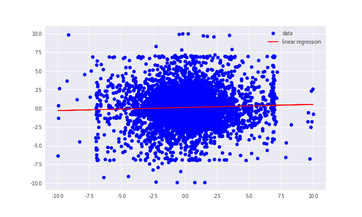
The summary report shows that the T statistics is greater than 2, so yesterday’s return(x1) has a significant effect on today’s return, so we should include x1 into our model.
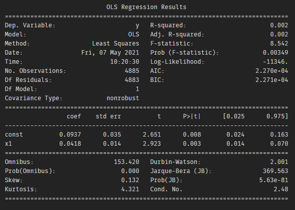
We think the information contains in x1 is not enough for us to well predicted the future return. Therefore, we adjust our model, consider more lag into the model. Finally, we take lag 2, 3-period return into account.

# 落後一期至三期的報酬率
data['R_t-1'] = data['報酬率%'].shift(1)
data['R_t-2'] = data['報酬率%'].shift(2)
data['R_t-3'] = data['報酬率%'].shift(3)
x = data[['R_t-1','R_t-2','R_t-3']][4:].values
y = data['報酬率%'][4:].values
reg_t3 = np.linalg.lstsq(x,y, rcond=None)[0]
# 繪圖
plt.figure(figsize=(10,6))
plt.plot(y[1000:1300],label = 'true_value')
plt.plot(np.dot(x, reg_t3)[1000:1300],color = 'green',label = 'predict')
plt.legend()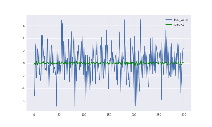
According to the summary report, the T statistics of x1 and x3 are higher than 2, so those two variables should include in our model.
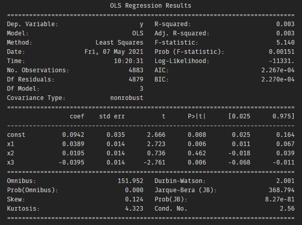
The part of linear regression has come to an end. Forecasting the market has always been a popular topic in finance and statistics. Interested friends can refer to relevant literature or explore other effective factors yourselves!!
Although logistic regression contains a regression in its name, it’s a kind of classification.
The difference between classification and regression their outputs. The classification outputs a discrete variable(such as 0,1,2, etc.);the regression outputs a continuous variable. (such as 0,0.1,0.5,1.2, etc.)
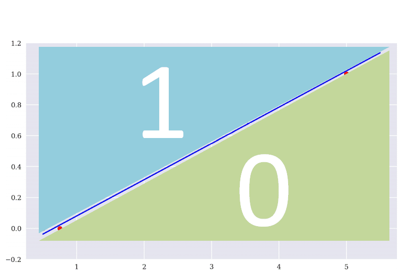
The concept of linear regression is to find a line whose average distance of points is minimization. The logistic regression aims to find a line that can classify data accurately the most. The illustrations below show the ideal condition, the model miss 2 in classify group 1, and miss 1 in classify group 0.
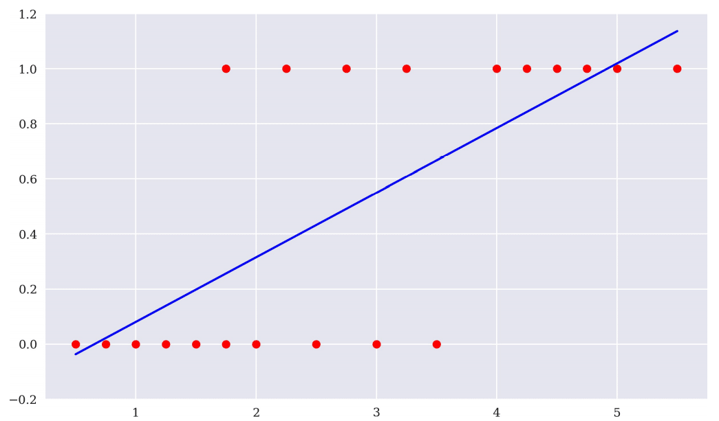
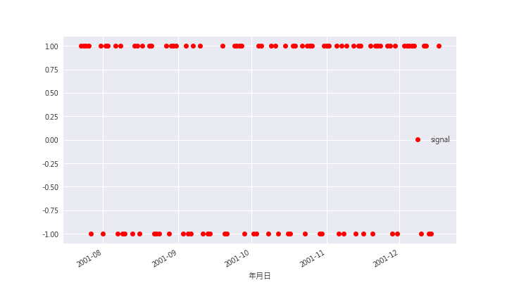
The predicting ability of the linear regression is not good, and hard to predict the actual value. Therefore, we try to simplify the problem. Change the target from its value to market movement(up and down). After all, if we could know the market movement tomorrow, we can construct a trading strategy.
np.where(condition, Ture(ouput), False(output)):
While return is higher than 0, ouput 1, otherwise, -1.
data['signal'] = np.where(data['報酬率%']>0,1,-1)
# 繪圖
data[:100].plot(x = '日期',
                y = 'signal',
                style = 'ro',
                figsize = (10,6)
               )
from sklearn import linear_model
lm = linear_model.LogisticRegression(solver = 'lbfgs')
R_t1 = x.reshape(1,-1).T
signal = y
lm.fit(R_t1,signal)
preditions = lm.predict(R_t1)
plt.figure(figsize = (10, 6))
plt.plot(x, y, 'ro', label = 'data')
plt.plot(x, preditions, 'b', label = 'preditions')
plt.legend(loc = 0)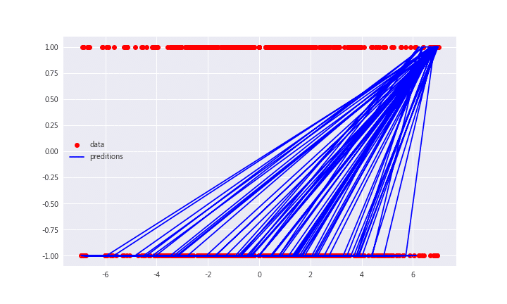
The accuracy of prediction is 0.5471.
from sklearn.metrics import accuracy_score
preditions = lm.predict(R_t1)
accuracy_score(preditions, y)After implement machine learning projection by yourself, did you find that it is difficult? 😎😎 Although the accuracy of the model is not high, don’t be discouraged about it. Predicting the market is not the only way to make money in the market. In the future, we will share the reasons why you can make money without prediction, so please pay attention to our Medium continuously.
If you like this topic, please click 👏 below, giving us more support and encouragement. Additionally, if you have any questions or suggestions, please leave a message or email us. We will try our best to reply to you.👍👍