Create a price deviation ratio trading strategy using python and perform historical backtesting.

Table of Contents
Article Difficulty: ★☆☆☆☆
Calculate the N-day Price Deviation Ratio Indicator using unadjusted closing prices of individual stocks and use the N-day previous low and high prices as entry and exit signals.
Reading Recommendation: This article primarily uses the Price Deviation Ratio and historical high and low points as entry and exit criteria. It provides a framework for readers to reference when conducting backtesting using programming.
The Price Deviation Ratio is a common technical indicator that compares the current stock price to the N-day moving average price, reflecting whether the current price is relatively high or low compared to its historical values. Generally, when the stock price consistently exceeds the moving average price, it’s called a ‘positive deviation.’ Conversely, it’s called’ negative deviation’ when it consistently falls below the moving average price.’ Therefore, when positive or negative deviation expands, it is interpreted as a sustained overbought or oversold condition in the market, serving as a basis for entry and exit decisions. However, using only the Price Deviation Ratio can generate too many trading signals. Hence, we include the highest and lowest prices over the past N days as a second filter. The actual strategy is as follows:
When the closing price is higher than the highest price over the past N days, and the Price Deviation Ratio is negative, enter a long position at the next day’s opening price.
When the closing price is lower than the lowest price over the past N days, and the Price Deviation Ratio is positive, exit the position and close the trade at the next day’s opening price.
This article uses Windows OS and employs Jupyter as the editor.
import tejapi as tej
import pandas as pd
import numpy as np
import datetime
import matplotlib.pyplot as plt
import ffn

tej.ApiConfig.api_key = 'Your Key'

plt.rcParams['font.family'] = 'Noto Sans TC'

%matplotlib inline
The data period is from 2015/01/05 to 2022/11/25, and for this example, we will retrieve unadjusted open, high, low, and close prices for TSMC (Taiwan Semiconductor Manufacturing Company).
#上市櫃公司代號

price = tej.get('TWN/APRCD',
                coid='2330',
                mdate={'gt': '2015-01-01', 'lt':'2022-11-28'},
                opts={'columns': ['coid', 'mdate', 'close_d', 'high_d', 'low_d', 'open_d']},
                chinese_column_name=True,
                paginate=True)


price['年月日'] = price['年月日'].dt.date
price = price.reset_index(drop=True)
After obtaining the stock prices, the first step is to calculate the Price Deviation Ratio (PD ratio) indicator. This is done by dividing the daily closing price by the moving average price over the past N days. It’s a good practice to write this calculation as a function for ease of parameter optimization in the subsequent steps.
def bias_cal(tmp ,n):

    df = tmp.copy()

    df['BIAS'] = ((df['收盤價(元)'] - df['收盤價(元)'].rolling(n).mean()) / df['收盤價(元)'].rolling(n).mean()).round(4)

    return df

bias_cal(price, 20).tail(10)
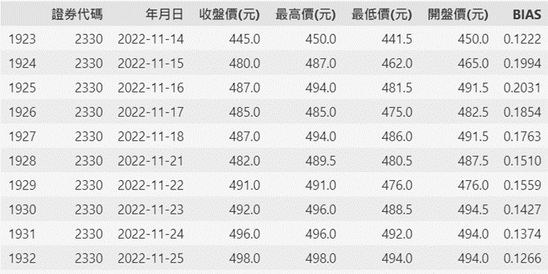
After calculating the price deviation ratio (PD ratio) for each day, historical backtesting is performed with the following transaction costs: buying commission of 0.1425%, and selling commission of 0.1425% plus a transaction tax of 0.3%. These calculations are encapsulated in functions to facilitate parameter optimization in the future.
def performance(tmp, n, init=1000000):
    df = tmp.copy()

    signal = 0

    df['his_low'] = df['最低價(元)'].shift(n)
    df['his_high'] = df['最高價(元)'].shift(n)

    df.loc[0, '現金'] = init
    df['進出場'] = 0

    for i in range(1, len(df)):

        if (df.loc[i-1, '收盤價(元)'] > df.loc[i-1, 'his_high']) & (df.loc[i-1, 'BIAS'] < 0) & (signal == 0):   #前一天收盤價小於n天前最低價,且收盤乖離率<=0,則當天開盤價進場

            df.loc[i, '股票'] =  df.loc[i, '開盤價(元)'] * 1000
            df.loc[i, '交易成本'] = round(-df.loc[i, '開盤價(元)']*1000*0.001425)
            df.loc[i, '現金'] = df.loc[i-1, '現金'] - df.loc[i, '股票'] + df.loc[i, '交易成本']
            df.loc[i, '進出場'] = '進場建倉'

            signal = 1

        elif (df.loc[i-1, '收盤價(元)'] < df.loc[i-1, 'his_low']) & (df.loc[i-1, 'BIAS'] > 0) & (signal == 1):   #前一天收盤價大於n天前最高價,且收盤乖離率>=0,則當天開盤價出場

            df.loc[i, '股票'] =  0
            df.loc[i, '交易成本'] = round(-df.loc[i, '開盤價(元)']*1000*0.004425)
            df.loc[i, '現金'] = df.loc[i-1, '現金'] + df.loc[i, '開盤價(元)']*1000 + df.loc[i, '交易成本']
            df.loc[i, '進出場'] = '出場平倉'

            signal = 0

        elif signal == 1:

            df.loc[i, '股票'] = df.loc[i, '收盤價(元)'] * 1000

            df.loc[i, '現金'] = df.loc[i-1, '現金']

        else:

            df.loc[i, '現金'] = df.loc[i-1, '現金']

    df['股票'] = df['股票'].fillna(0)
    df['交易成本'] = df['交易成本'].fillna(0)
    df['總權益'] = df['現金'] + df['股票']

    print('總權益:', df['總權益'].iloc[-1])
    print('交易成本:', df['交易成本'].sum())
    print('報酬率:', '%.2f'%((df['總權益'].iloc[-1] - init)/init*100), '%')

    print('年均報酬率:', '%.3f'%(df['總權益'].pct_change().mean()*252*100), '%')
    print('年化標準差:', '%.3f'%(df['總權益'].pct_change().std()*np.sqrt(252)*100), '%')
    print('夏普值:', '%.3f'%((df['總權益'].pct_change().mean()*252*100) / (df['總權益'].pct_change().std()*np.sqrt(252)*100)))

    print('最大回撤:', '%.2f'%(((df['總權益'] / df['總權益'].cummax() - 1).cummin().iloc[-1])*100), '%')

    return df

result = performance(bias_cal(price, 20), 20)
首先用一個月20天,起始金額100萬為參數來看看成果,可以看出到了最後一天只剩下90萬,其中大部分都被交易成本給耗光了,只賺到微幅的報酬1.17%。
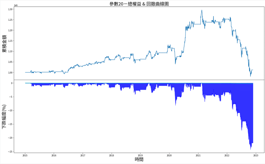
Visualizing the total equity and drawdown curve, we can see the results. It’s evident that starting from mid-2021, there was a significant upward trend with TSMC. However, in recent times, due to factors like interest rate hikes and the Ukraine-Russia conflict, it has experienced its largest drawdown to date, giving back some of the previous gains.
n = 20
result = performance(bias_cal(price, n), n)
fig, ax = plt.subplots(2, 1, figsize=(20, 12), sharex=True)

ax[0].plot(result['年月日'], result['總權益'])

ax[1].plot(result['年月日'], result['總權益'].to_drawdown_series().to_list(), color='c')

dd = (result['總權益'].to_drawdown_series()*100).to_list()

ax[1].fill_between(result['年月日'], np.zeros(len(result['總權益'])), dd, label='大盤 DD', color='blue', linewidth=1, alpha=0.8)

ax[0].set_title(f'參數{n}-總權益 & 回撤曲線圖', fontsize=20)
ax[1].set_xlabel('時間', fontsize=20)

ax[0].set_ylabel('累積金額', fontsize=20)
ax[1].set_ylabel('下跌幅度(%)', fontsize=20)


plt.subplots_adjust(hspace=.0)
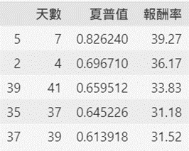
In the subsequent steps, we further optimize the parameters to find the best N days, ranging from 2 days to 50 days, selecting the parameter that results in the highest Sharpe ratio.
optim = []
for i in range(2, 51):
    df = performance(bias_cal(price, i), i)

    sharp = ((df['總權益'].pct_change().mean()*252) / (df['總權益'].pct_change().std()*np.sqrt(252)))

    ret = round(((df['總權益'].iloc[-1] / df['總權益'].iloc[0]) - 1), 4)*100

    optim.append((i, sharp, ret))

    result1 = pd.DataFrame(optim, columns=['天數', '夏普值', '報酬率'])

result1.sort_values('夏普值', ascending=False).head(5)
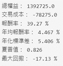
After optimizing with different parameters, it was found that a 7-day calculation period performed the best in historical backtesting.
result = performance(bias_cal(price, 7), 7)
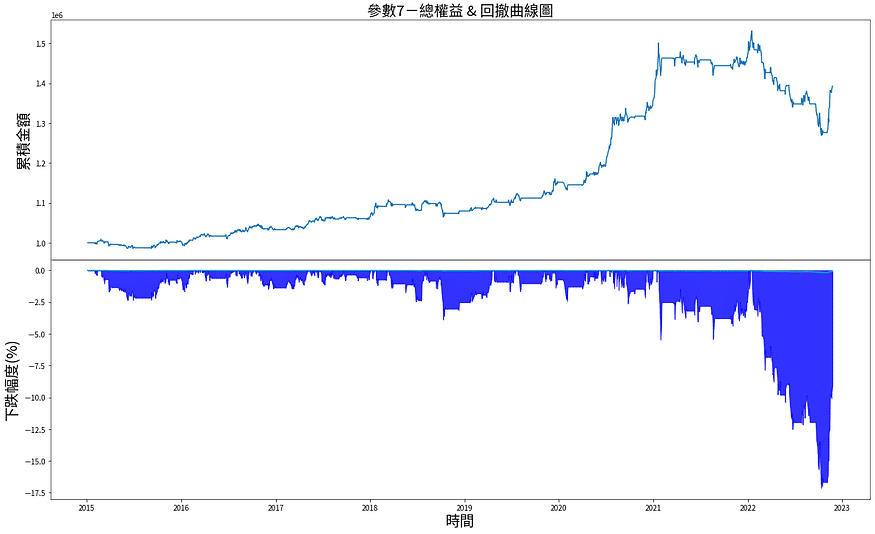
The overall Sharpe ratio has improved from 0.055 to 0.826, and the return rate has increased significantly to nearly 40%. Additionally, the maximum drawdown has also decreased significantly.

From the equity curve, it can be seen that the strategy had good performance around the beginning of 2022 but was ultimately unable to withstand the recent strong interest rate hikes, resulting in the largest drawdown since 2015.
The strategy introduced in this session is one of the mean-reversion trading strategies. When the market is oversold (Bullish Divergence, BDI < 0), and the closing price is higher than the highest price over a certain period, it’s assumed that the stock price will gradually return to the moving average price, so a long position is entered. Conversely, when the stock price is overbought (Bearish Divergence, BDI > 0), and the closing price is lower than the lowest price over a certain period, it’s believed that the stock price has risen too much and has a downward trend. In this case, the long position is exited. However, it’s important to note that this strategy involves frequent trading, which can be eroded by transaction costs and taxes. Therefore, it’s recommended to combine other technical indicators to optimize entry and exit points.
Finally, it’s worth mentioning again that the stocks discussed in this article are for illustrative purposes only and do not constitute recommendations for any financial products. If readers are interested in topics such as building strategies, performance backtesting, and empirical research, you are welcome to purchase solutions from TEJ E-Shop, which provides comprehensive databases to easily perform various tests and analyses.