
Fulfill Roger E. King’ s investing strategy through python.
Table of Contents
Roger E. King is a well-known value fund manager in the United States. He used to be the senior vice president and chief investment officer of Sun Insurance Services and senior vice president of GULFCO Investment Management. He founded King Investment Advisors Inc. in 1981. By 2001, he had an investment experience of 30 years.
Originally, King Investment Consultants only managed institutional investors’ funds and individual retirement funds. At the end of 1996, it issued the first stock mutual fund-Fountainhead Special Value Fund. It was a blockbuster in 1997 and received 36.65% of investment returns. In 1999, the return on investment reached 133.44%. Although the stock market performed poorly in 2000, the fund performance only lost 15.71%. As of May 2001, the 3-year average return rate reached 18.22%, surpassing the performance of the S&P 500 index by 12.92% over the same period. As a result, it has received a 5-star rating from the Morning star Co. Fund, and its investment performance is very good.
He developed a stock selection strategy called “Business Valuation Approach” by himself, which is based on the bottom-up stock selection method, which is divided into three valuation methods:
(1) Private-market Valuation, Liquidation or acquired in a cash transaction;
(2) Historical Valuation;
(3) Superior Earning Growth, Buy growth at a reduced price: GARP
The companies selected by the three methods can all be investment targets, which are then screened based on indicators such as financial strength and insider entry and exit; although Roger King is positioned as a value investor by the market, he emphasized that buying has investment value. In an interview with the media, he once said, “The secret of success is to buy at an inexpensive price (The secret of success is to buy at an inexpensive price). This time I introduce the second stock selection method “History Evaluation”.
All the indicators below were calculated by 7-year historical data to determine the potential upside return and potential downside risk.
Average of highest and lowest PE ratio per 7 years.
Average of highest and lowest PB ratio per 7 years.
Average of highest and lowest PCF ratio per 7 years.
Average of highest and lowest PS ratio per 7 years.
Solid financial condition.
Shareholder of internal staff .
To calculate the average highest and lowest PE, PB, PCF, and PS ratio, we will have to find the highest and lowest point each year, then take an average of them. To determine whether to buy the stocks, we estimate the potential upside and downside through the indicators.
For the change in time and location, we made an adjustment to the above conditions.
PE ratio upside target price = 7-year average of highest PE ratio * recent EPS
PE ratio downside target price = 7-year average of lowest PE ratio * recent EPS
PB ratio upside target price = 7-year average of highest PB ratio * recent book value
PB ratio downside target price = 7-year average of lowest PB ratio * recent book value
PCF ratio upside target price = 7-year average of highest PCF ratio * recent cash flow
PCF ratio downside target price = 7-year average of lowest PE ratio * recent cash flow
PS ratio upside target price = 7-year average of highest PS ratio * recent sales revenue
PS ratio downside target price = 7-year average of lowest PS ratio * recent sales revenue
Standards of stock selection:
The standards below shows the distance between stock price and downside target price, the closer means the stock is under value and have a greater potential return.
PE return/risk ratio = [(PE ratio upside target price- recent stock price)/(recent stock price – PE ratio downside target price)]>1
PB return/risk ratio = [(PB ratio upside target price- recent stock price)/(recent stock price – PB ratio downside target price)]>1
PCF return/risk ratio = [(PCF ratio upside target price- recent stock price)/(recent stock price – PCF ratio downside target price)]>1
PS return/risk ratio = [(PS ratio upside target price- recent stock price)/(recent stock price – PS ratio downside target price)]>1
If one of the above 4 indicators is met, it is the stock selection target. Additional filter by the following conditions:
kick off the stock with debt to asset ratio in most recent quarter > 65%.
Roger King’s return/risk ratio measured the distance among the recent stock price, upside target price, and downside target price. If the stock price is closer to the downside target price than the upside target price, it means the stock is cheap now, vice versa. According to the aim of value investment, we will buy the undervalued one.
import pandas as pd
import numpy as np
import matplotlib.pyplot as plt
plt.style.use('seaborn')
import tejapi
tejapi.ApiConfig.api_key = 'your_key'
tejapi.ApiConfig.ignoretz = True# 獲取上市普通股代碼 #
stk_info = tejapi.get('TWN/ANPRCSTD',
paginate=True,
chinese_column_name=True
)
stk_nums = stk_info[(stk_info['上市別']=='TSE') & (stk_info['證券種類名稱']=='普通股')]['證券碼'].to_list()
# 撈取財務資料 #
zz = pd.DataFrame()
for code in stk_nums:
zz = zz.append(
tejapi.get('TWN/AIM1A',
coid=code,
paginate=True,
chinese_column_name=True,
opts= {'pivot':True,'columns':['coid','mdate','200D','R535','R505','R303','R304','MV']}).reset_index(drop=True)
).reset_index(drop=True)
print(code)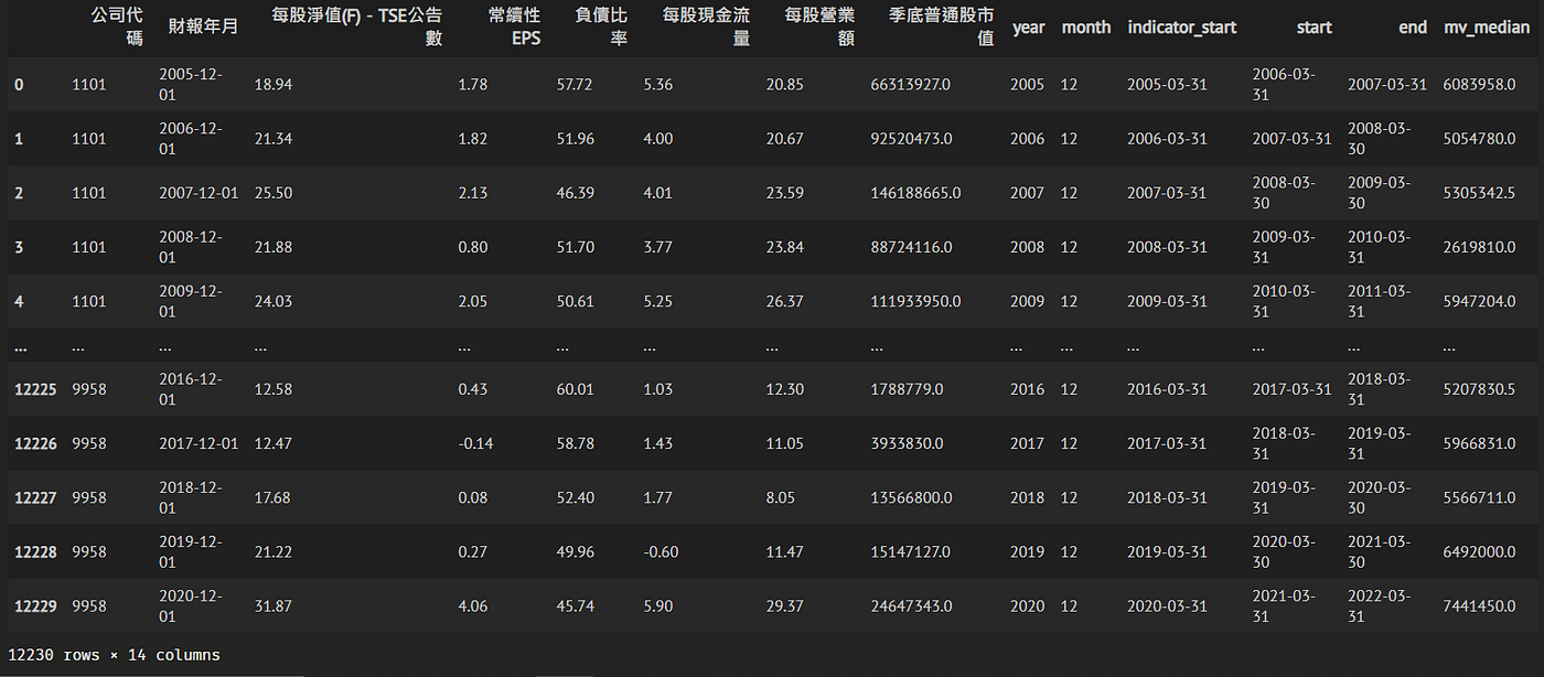
Tips : The way to find the codes of the wanted column. Just enter the keyword and run the code below, tejapi will help to search for you.
# IFRS財務會計科目說明檔 #
acc = tejapi.get(‘TWN/AIACC’,paginate=True)
# 搜尋欄位代碼 #
key_word = '輸入關鍵字'
acc[acc[‘cname’].str.find(key_word)!=-1]For example, when calculating PE, PB, PCF, and PS at the end of 2010–12–31, we use the stock price from 2010–3–31 to 2011–3–31.
PS. The run time is about 40 minutes.
results = pd.DataFrame()
#coid = str(1101)
for coid in data['公司代碼'].unique():
    stock = tejapi.get('TWN/APRCD1',coid = coid, chinese_column_name = True)
    for year in data['year'].unique():
        condition = (data['year']==year) & (data['公司代碼']== coid)
        if (data[condition].size !=0):
            indicator_start = data['indicator_start'][condition].to_list()[0]
            stk_start = data['start'][condition].to_list()[0]
            stk_end = data['end'][condition].to_list()[0]
            # 抓取財報季度前一年的資料 #
            selected = stock[(stock['年月日'] > indicator_start) & (stock['年月日'] < stk_start)].reset_index(drop=True)
            back_test = stock[(stock['年月日'] >= stk_start) & (stock['年月日'] < stk_end)].reset_index(drop=True)
            if (selected.size!=0) and (back_test.size!=0):
                # 計算個年度最高與最低 本益比、股價淨值比、股價現金流量比和股價營收比 #
                price = selected['收盤價(元)'].tail(1).to_list()[0]
                stk_start_price = back_test['收盤價(元)'].head(1).to_list()[0]
                ## 本益比 ##
                EPS = data['常續性EPS'][condition].to_list()[0]
                PE = selected['收盤價(元)']/EPS
                PE_max = PE.max()
                PE_min = PE.min()
                ## 股價淨值比 ##
                BV = data['每股淨值(F)-TSE公告數'][condition].to_list()[0]
                PB = selected['收盤價(元)']/BV
                PB_max = PB.max()
                PB_min = PB.min()
                ## 股價現金流量比 ##
                CFP = data['每股現金流量'][condition].to_list()[0]
                PC = selected['收盤價(元)']/CFP
                PC_max = PC.max()
                PC_min = PC.min()
                ## 股價營收比 ##
                SP = data['每股營業額'][condition].to_list()[0]
                PS = selected['收盤價(元)']/SP
                PS_max = PS.max()
                PS_min = PS.min()
                # 彙整 #
                result = pd.DataFrame({
                    'year':year,
                    '公司代碼':coid,
                    'stk_start':stk_start,
                    'stk_end':stk_end,
                    'stk_start_price':stk_start_price,
                    'PE_max':PE_max,'PE_min':PE_min,
                    'PB_max':PB_max,'PB_min':PB_min,
                    'PC_max':PC_max,'PC_min':PC_min,
                    'PS_max':PS_max,'PS_min':PS_min
                },index=[0])
                results = results.append(result).reset_index(drop=True)
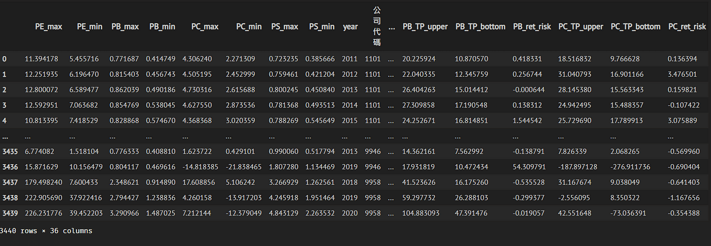
print(coid)Using the result of maximum and minimum of PE, PB, PCF, and PS each year to compute the 7-year rolling mean. Also, combine the the most recent EPS, book value, cash flow, and sales revenue. Finally, we will get the upside target price, downside target price, and return risk ratio.
mean_7 = results.groupby(by=['公司代碼']).rolling(7).mean()[['PE_max','PE_min','PB_max','PB_min','PC_max','PC_min','PS_max','PS_min']]
mean_7 = mean_7.reset_index(drop=True)
mean_7['year'],mean_7['公司代碼'],mean_7['stk_start_price'] = results['year'], results['公司代碼'],results['stk_start_price']
# 合併 #
mean_7 = pd.merge(mean_7.dropna(),data,on=['公司代碼','year'])
# 去除市值小於中位數者 #
mean_7 = mean_7[(mean_7['季底普通股市值']>mean_7['mv_median'])].reset_index(drop=True)
PE return/risk ratio = [(PE ratio upside target price- recent stock price)/(recent stock price — PE ratio downside target price)]>1
PB return/risk ratio = [(PB ratio upside target price- recent stock price)/(recent stock price — PB ratio downside target price)]>1
PCF return/risk ratio = [(PCF ratio upside target price- recent stock price)/(recent stock price — PCF ratio downside target price)]>1
PS return/risk ratio = [(PS ratio upside target price- recent stock price)/(recent stock price — PS ratio downside target price)]>1
If one of the above 4 indicators is met, it is the stock selection target. Additional filter by the following conditions:
kick off the stock with debt to asset ratio in most recent quarter > 65%.
# 目標價計算 #
## 本益比 ##
mean_7['PE_TP_upper'] = mean_7['PE_max']*mean_7['常續性EPS']
mean_7['PE_TP_bottom'] = mean_7['PE_min']*mean_7['常續性EPS']
mean_7['PE_ret_risk'] = (mean_7['PE_TP_upper']-mean_7['stk_start_price'])/(mean_7['stk_start_price']-mean_7['PE_TP_bottom'])
## 股價淨值比 ##
mean_7['PB_TP_upper'] = mean_7['PB_max']*mean_7['每股淨值(F)-TSE公告數']
mean_7['PB_TP_bottom'] = mean_7['PB_min']*mean_7['每股淨值(F)-TSE公告數']
mean_7['PB_ret_risk'] = (mean_7['PB_TP_upper']-mean_7['stk_start_price'])/(mean_7['stk_start_price']-mean_7['PB_TP_bottom'])
## 股價現金流量比 ##
mean_7['PC_TP_upper'] = mean_7['PC_max']*mean_7['每股現金流量']
mean_7['PC_TP_bottom'] = mean_7['PC_min']*mean_7['每股現金流量']
mean_7['PC_ret_risk'] = (mean_7['PC_TP_upper']-mean_7['stk_start_price'])/(mean_7['stk_start_price']-mean_7['PC_TP_bottom'])
## 本益比 ##
mean_7['PS_TP_upper'] = mean_7['PS_max']*mean_7['每股營業額']
mean_7['PS_TP_bottom'] = mean_7['PS_min']*mean_7['每股營業額']
mean_7['PS_ret_risk'] = (mean_7['PS_TP_upper']-mean_7['stk_start_price'])/(mean_7['stk_start_price']-mean_7['PS_TP_bottom'])
# 評分 #
mean_7.loc[:,'score'] = 0
mean_7['score'] = np.where(mean_7['PE_ret_risk'] > 1, 1+mean_7['score'], mean_7['score'])
mean_7['score'] = np.where(mean_7['PB_ret_risk'] > 1, 1+mean_7['score'], mean_7['score'])
mean_7['score'] = np.where(mean_7['PC_ret_risk'] > 1, 1+mean_7['score'], mean_7['score'])
mean_7['score'] = np.where(mean_7['PS_ret_risk'] > 1, 1+mean_7['score'], mean_7['score'])

%%time
return_=pd.DataFrame()
for year in range(2011,2020):
    pf = mean_7[(mean_7['year']==year) & (mean_7['負債比率'] < 65) & (mean_7['score']>=1)]#.sort_values(by = 'score', ascending = False).reset_index(drop=True)
    ## 將買進日期設在季底+90日 ##
    buy_date = mean_7['start'][mean_7['year']==year].head(1).to_list()[0]
    sell_date = mean_7['end'][mean_7['year']==year].head(1).to_list()[0]
    ret = pd.DataFrame()
    pf_H = pf['公司代碼'].to_list()
    print('投資組合共有{}檔股票'.format(len(pf_H)))
    ## 自 tejapi撈取日報酬資料,日期設定為 buy_date(不含)至 sell_date(含) ##
    print('getting data')
    stk_data = tejapi.get('TWN/APRCD2',
                          coid = pf_H,
                          paginate = True,
                          mdate={'gt':buy_date,'lt':sell_date},
                          chinese_column_name=True)
    # 計算報酬率 #
    print('calculating return')
    pf_ret = stk_data.groupby(by = '年月日').mean()['日報酬率 %']
    pf_ret = pf_ret.reset_index(drop=True)
#     ret[ranking[i]] = pf_ret
    ret['portfolio'] = pf_ret
#     i+=1
    ## 撈取台灣加權指數的日報酬率,日期設定為 buy_date(不含)至 sell_date(不含) ##
    twse = tejapi.get('TWN/APRCD2',coid ='Y9999' ,paginate = True,mdate={'gt':buy_date,'lt':sell_date},chinese_column_name=True)
    bm_return = twse.groupby('年月日').mean()['日報酬率 %'].reset_index(drop=True)
    ret['twse_return'] = bm_return
    ret['Date'] = twse['年月日']
    return_ = return_.append(ret).reset_index(drop=True)
    print(return_)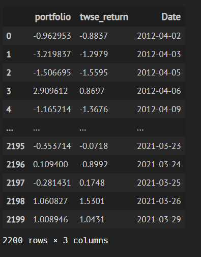
cum_ret = return_[['portfolio','twse_return']].astype(float).apply(lambda x:x*0.01+1).cumprod().reset_index(drop=True)
cum_ret['Date'] = return_['Date']
cum_ret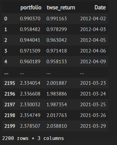
cum_ret.plot(x='Date',figsize=(10,6))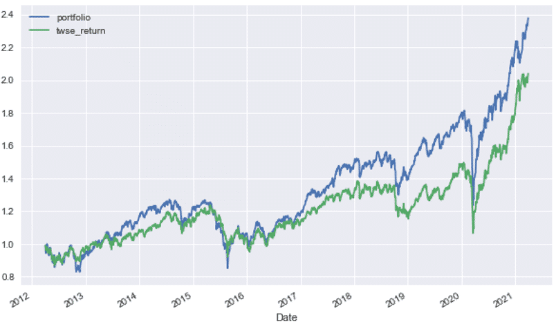
# 績效報表 #
yearly_mean_ret = (((cum_ret[['portfolio','twse_return']].tail(1)**(1/len(cum_ret)))**252-1)*100).reset_index(drop=True)
yearly_std = cum_ret[['portfolio','twse_return']].std()*(252**(0.5))
Rf = 1
sp_ratio = (yearly_mean_ret-Rf)/yearly_std
roll_max = cum_ret[['portfolio','twse_return']].cummax()
draw_down = (cum_ret[['portfolio','twse_return']]-roll_max)/roll_max
MDD = draw_down.min()*100
performace_report = pd.DataFrame({
    'portfolio':[yearly_mean_ret['portfolio'].values[0],
                 yearly_std['portfolio'],
                 sp_ratio['portfolio'].values[0],
                 MDD['portfolio']],
    'twse_return':[yearly_mean_ret['twse_return'].values[0],
                   yearly_std['twse_return'],
                   sp_ratio['twse_return'].values[0],
                   MDD['twse_return']]}
    ,index= ['年化報酬','年化波動度','夏普指標','最大回檔'])
performace_report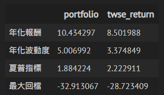
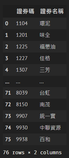
pf2020 = mean_7[(mean_7['year']==2020) & (mean_7['負債比率'] < 65) & (mean_7['score']>=1)]['公司代碼'].to_list()
stk_info[['證券碼','證券名稱']][stk_info['證券碼'].isin(pf2020)].reset_index(drop=True)
Our portfolio outperforms the twse index at the aspect of cumulative return, but after taking risk into account, the benchmark beats the portfolio at volatility, Sharpe ratio, and max drawdown.
Roger King’s investing strategy wins the benchmark by a narrow margin at return, but fail to exceed the benchmark after considering the risk. The result is quite different as our expect, however there doesn’t have a stable holy grail for the long-time, all the criteria should adjust along with time.
The most important is to extract thinking and experience from the investment master like Roger King and Benjamin Graham. Finally, construct your own strategy.
Next time, we will share the investing concept of Trinity Investment Management !!
Finally, if you like this article, please click below, giving us more support and encouragement. Besides, if you have any questions or suggestions, please leave a message or email us, we will try our best to reply to you.