Use common technical indicators to backtesting

Table of Contents
Relative strength index (RSI) is the momentum technical indicator. It is usually used as an oscillator interval to evaluate overbought or oversold condition by measuring recent trend of price movements. Following is the way to calculate this indicator:
Criterion of RSI:
RSI’s Deactivation: Gain and loss is separately calculated in RSI. Therefore, if short-term trend of price is almost gain, the reference data of loss would be too few to be considered, which further causes that RSI loses the reference value, vice versa. This situation is specifically frequent during the high or low-level area. We would try to synthesize RSI interval, golden cross and death cross to lower the impact of deactivation.
MacOS and Jupyter Notebook
#Basic function
import pandas as pd
import numpy as np
import copy#Visualization
import plotly.graph_objects as go
import plotly.express as px#TEJ
import tejapi
tejapi.ApiConfig.api_key = 'Your Key'
tejapi.ApiConfig.ignoretz = True
Step 1. Obtain the stock price
stock_data = tejapi.get('TWN/APRCD',
           coid= '2324', # Compal Electronics, Inc.
           mdate={'gte': '2020-01-01', 'lte':'2021-12-14'},
           opts={'columns': ['coid', 'mdate', 'open_d', 'close_d']},
           chinese_column_name=True,
           paginate=True)
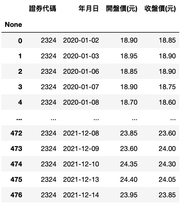
We choose Compal Electronics (2324) as the target. Time interval is ranged from 2020 to today (2021–12–14). With above circumstances, we would know the fluctuation of stock price of largest notebook OEM under the pandemic situation. On top of that, determine the buy and sell signal with RSI.
Step 2. Calculate 14-day RSI & 7-day RSI
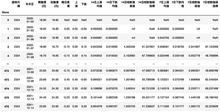
# Calculate daily spread and categorize gain & loss
stock_data['隔日差價'] = stock_data['收盤價(元)'].diff()
stock_data['上漲'] = stock_data['隔日差價'].clip(lower = 0)
stock_data['下跌'] = (-1) * stock_data['隔日差價'].clip( upper = 0)# 14-day RSI
stock_data['14日上漲均值'] = stock_data['上漲'].ewm(com = 14, adjust = False).mean()
stock_data['14日下跌均值'] = stock_data['下跌'].ewm(com = 14, adjust = False).mean()
stock_data['14日相對強弱值'] = stock_data['14日上漲均值'] / stock_data['14日下跌均值']
stock_data['14日相對強弱指標'] = stock_data['14日相對強弱值'].apply(lambda rs : rs/(1+rs)*100)# 7-day RSI
stock_data['7日上漲均值'] = stock_data['上漲'].ewm(com = 7, adjust = False).mean()
stock_data['7日下跌均值'] = stock_data['下跌'].ewm(com = 7, adjust = False).mean()
stock_data['7日相對強弱值'] = stock_data['7日上漲均值'] / stock_data['7日下跌均值']
stock_data['7日相對強弱指標'] = stock_data['7日相對強弱值'].apply(lambda rs : rs/(1+rs)*100)
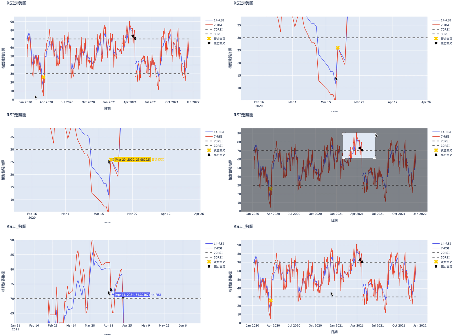
Step 3. RSI Trending Chart & Interval (30,70)(See the details in source code)
Comparing RSI trending and overbought, oversold interval, we find the Golden Cross and Death Cross. What we should notice is that deactivation remains serious at the high-level area. However, we should sell at the first death cross, since it is impossible to predict market accurately.
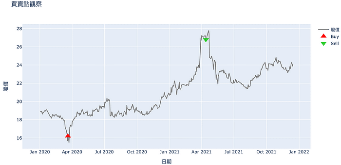
Step 4. Find Buy and Sell Signal & Visualize Trading Action(See the details in source code)
Over-sold Condition: RSI < 30. To boot, consider that 7-day RSI exceeds 14-day RSI upwards so as to lower impact of low-level deactivation.
Over-bought Condition: RSI > 70. To boot, consider that 7-day RSI exceeds 14-day RSI downwards so as to lower impact of high-level deactivation.
signal = []trade = 0for i in range(len(stock_data)):
    if stock_data.loc[i, '14日相對強弱指標']  <= 30 and stock_data.loc[i-1, '14日相對強弱指標'] > stock_data.loc[i-1, '7日相對強弱指標'] and stock_data.loc[i, '14日相對強弱指標'] <= stock_data.loc[i, '7日相對強弱指標'] and trade == 0:        signal.append(1000)
        trade = trade + 1    elif stock_data.loc[i, '14日相對強弱指標'] >= 70 and stock_data.loc[i-1, '14日相對強弱指標'] < stock_data.loc[i-1, '7日相對強弱指標'] and stock_data.loc[i, '14日相對強弱指標'] >= stock_data.loc[i, '7日相對強弱指標'] and trade == 1:        signal.append(-1000)
        trade = trade - 1    else:
        signal.append(0)stock_data['買賣股數'] = signal
In 【Quant(8)】Backtesting by MACD Indicator, we have discussed the details in the calculation of frictions cost and the method to calculate return with initial principal. In this article, we use function to achieve all of it.
def target_return(data, principal):

    #計算成本
    data['手續費'] = data['開盤價(元)']* abs(data['買賣股數'])*0.001425
    data['手續費'] = np.where((data['手續費']>0)&(data['手續費'] <20), 20, data['手續費'])
    data['證交稅'] = np.where(data['買賣股數']<0, data['開盤價(元)']* abs(data['買賣股數'])*0.003, 0)
    data['摩擦成本'] = (data['手續費'] + data['證交稅']).apply(np.floor)

    #計算資產價值
    data['股票價值'] = data['買賣股數'].cumsum() * data['收盤價(元)']
    data['現金價值'] = principal - data['摩擦成本'] + (data['開盤價(元)']* -data['買賣股數']).cumsum()
    data['資產價值'] = data['股票價值'] + data['現金價值']

    #計算報酬率
    data['當日價值變動(%)'] = (data['資產價值']/data['資產價值'].shift(1) - 1)*100
    data['累計報酬(%)'] = (data['資產價值']/principal - 1)*100

    return data
We only consider the trading of common stock. There is no margin buy or margin sell situation, so we do not have to calculate premium. With the data containing trading shares and initial principal, we can quickly get the transaction costs and return. In this article, we set 20,000 as our principal
RSI_return = target_return(data = stock_data, principal = 20000)
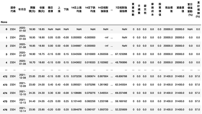
Besides, to demonstrate whether RSI strategy performs relatively well, we add buy-and-hold strategy and market performance as our benchmarks.
bh_data = copy.deepcopy(stock_data)
bh_data['買賣股數'] = 0
bh_data.loc[0, '買賣股數'] = 1000
bh_data.loc[len(bh_data)-1, '買賣股數'] = -1000# Drop the columns useless for buy-and-hold calculation.
bh_data = bh_data.drop(['隔日差價', '上漲', '下跌', '14日上漲均值', '14日下跌均值', '14日相對強弱值','14日相對強弱指標','7日上漲均值', '7日下跌均值', '7日相對強弱值', '7日相對強弱指標'], axis = 1)bh_return = target_return(data=bh_data, principal = 20000)
Here we also use deepcopy() to get stock price, and choose to buy at the beginning and sell at the end during the same period with initial principal of 20000 as well.
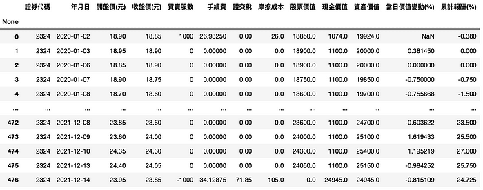
market = tejapi.get('TWN/APRCD',
                   coid = 'Y9997',
                   mdate = {'gte':'2020-01-01', 'lte':'2021-12-14'},
                   opts = {'columns':['coid','mdate',   'close_d','roi']},
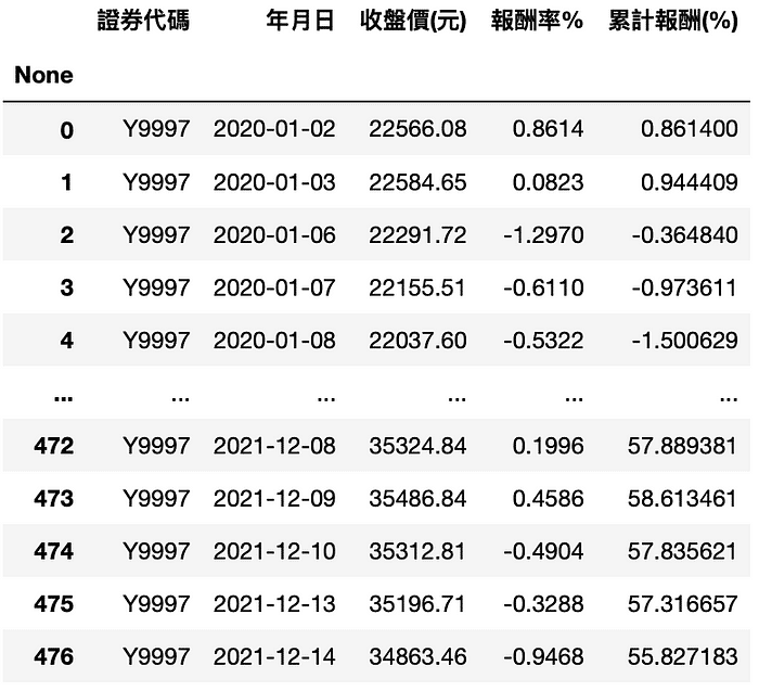
                   chinese_column_name = True)market['累計報酬(%)'] = (market['報酬率%'].apply(lambda x:0.01*x +1).cumprod() - 1)*100
Obtain return of market return index (Y9997) to stands for market performance and calculate the cumulative return
Step 1. Comparison of cumulative return (See the details in source code)
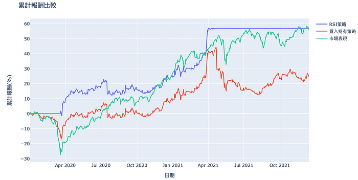
With the chart of cumulative return, We tell that RSI strategy made us long after the pandemic. As for the short position, RSI made us sell right at the point that electronic-related stocks were shorted, which was caused by the rise of Commodity’s price and market, therefore, focused on traditional stocks. Besides, fortunately, we avoid the impact of abruptly Covid’s intensification in Taiwan. However, due to the standard of signal trigger is strict, we cannot accurately handle every fluctuation period, like the drop during Aug 2020.
Step 2. Performance table (See the details in source code)
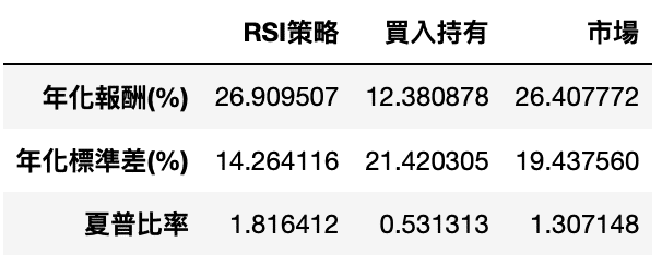
Above chart shows that RSI strategy outperforms buy-and-hold on both return and volatility, which means that RSI helps us find adequate long and short point and improve the efficiency of investment. As for the comparison with market, return of RSI does not outperform market return significantly, but the volatility of RSI is relatively stable. Resulting from avoiding pandemic crash in 2020 and local crash in Taiwan in 2021, sharpe ratio of RSI is better than market performance.
With the above content, we believe readers understand the influence of deactivation, especially during high or low-level area. Hence, we add another condition, cross of long-term and short-term RSI, making RSI strategy more steady. Of course, on the other hand, this sacrifices some trading opportunities. The balance between risk and trading opportunities is what investors should evaluate and strike. After all, the application of technical indicator varies from person to person. As a result, if readers are interested in diverse trading backtesting, welcome to purchase the plan offered in TEJ E-Shop. Construct trading strategies fitting you with high quality database.