The alpha obtained from the Fama&French three-factor model is used to construct a long-short strategy and backtest the performance against the market return.

Table of Contents
Difficulty:★★☆☆☆
The Fama&French three-factor model is used to calculate the alpha of Taiwan-listed stocks, and the top 20% of stocks with the highest alpha and the bottom 20% of stocks with the lowest alpha are obtained to make a long-short strategy portfolio and evaluate the performance.
This article will start with the establishment of the three-factor model to calculate the SMB and HML. Therefore, it is necessary to have a preliminary understanding of the Capital Asset Pricing Model (CAPM) in investment and to understand the concept of alpha and beta, which will be more helpful to read the article.
The Capital Asset Pricing Model (CAPM) occupies an important position in Modern Portfolio theory and is the basis of modern financial market price theory, and many scholars have continued to extend on this basis and created various factor models, and there is even a factor zoo. For example, Fama & French’s three-factor model used in this paper is to add a size premium and a B/M ratio premium to the CAPM, which only considers the market factor, in order to expect the return of the portfolio or stock to be explained by these three factors.
This article uses Mac OS as system and jupyter as editor.
import pandas as pd
import numpy as np
import tejapi
import statsmodels.api as sm
import matplotlib.pyplot as plt
import matplotlib.transforms as transforms
plt.rcParams['font.sans-serif'] = ['Arial Unicode MS'] # 解決MAC電腦 plot中文問題
plt.rcParams['axes.unicode_minus'] = False
tejapi.ApiConfig.api_key ="Your Key"
tejapi.ApiConfig.ignoretz = True
Listed company adjusted stock price(daily)-ex-right and dividends adjustment (TWN/APRCD1)
Securities Property Information(TWN/ANPRCSTD)
Data was obtained for the period from January 2014 to June 2021 for listed stock codes, closing prices, return, market capitalization, and price-to-book ratio.
data=tejapi.get('TWN/ANPRCSTD' ,chinese_column_name=True )
select=data["上市別"].unique()
select=select[1:3]
condition =(data["上市別"].isin(select)) & ( data["證券種類名稱"]=="普通股" )
data=data[condition]
twid=data["證券碼"].to_list()  #取得上市櫃股票證券碼

df = pd.DataFrame()
for i in twid: #資料筆數超過100萬筆,透過迴圈方式抓取
    df = pd.concat([df, tejapi.get('TWN/APRCD1',  #從TEJ api撈取所需要的資料
                  chinese_column_name = True,
                  paginate = True,
                  mdate = {'gt':'2013-12-31', 'lt':'2022-07-01'},
                  coid=i,
                  opts={'columns':['coid','mdate', 'close_adj' ,'roi' ,'mv', "pbr_tej"]})])
The book-to-market ratio is obtained by first taking the inverse of the price-to-book ratio, then obtaining the median daily market capitalization, and label stocks larger than the median as B and those smaller than the median as S to form two portfolios.
df['帳面市值比'] = 1/df['股價淨值比-TEJ']

ME = df.groupby('年月日')['市值(百萬元)'].apply(lambda x: x.median())
ME.name = '市值_中位數'
df = df.merge(ME, on='年月日')
df['市值matrix'] = np.where(df['市值(百萬元)']>df['市值_中位數'], 'B', 'S')
The weight of the portfolio is obtained by weighting the large-cap portfolio and the small-cap portfolio by value weighted, and confirming whether the total weight of both portfolios is equal to 1.
df1 = (df.groupby(['年月日','市值matrix'])['市值(百萬元)'].sum()).reset_index()
df = df.merge(df1, on=['年月日','市值matrix'])
df['weight'] = df['市值(百萬元)_x']/df['市值(百萬元)_y']
df.groupby(['年月日','市值matrix'])['weight'].sum()

df.groupby(['年月日','市值matrix'])['weight'].sum()
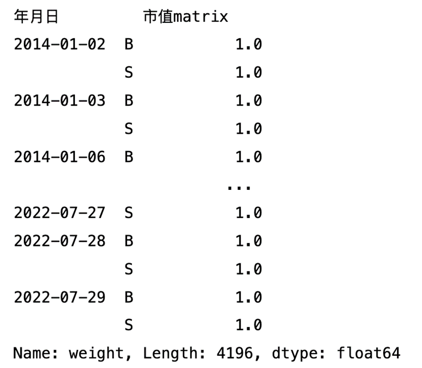
The SMB factor is calculated by subtracting the return on the big-cap portfolio from the return on the small-cap portfolio to form a long-short portfolio.
df['return1'] = df['報酬率%']* df['weight']
SMB = df.groupby(['年月日','市值matrix'])['return1'].sum()
SMB.reset_index(inplace=True)
SMB.set_index('年月日',drop=True, inplace=True)
SMB = SMB[SMB['市值matrix']=='S']['return1'] - SMB[SMB['市值matrix']=='B']['return1']
SMB.name = 'SMB'
SMB
Fama&French divided the BM ratio into 30%, 40%, and 30%, so I obtained the BM ratio of the 30th percentile and 70th percentile and labeled those larger than the 70th percentile as V(value), those smaller than 30% as G(growth), and the rest as N(Neutral) to form three portfolios.
a = df.groupby('年月日')['帳面市值比'].quantile(0.7)
a.name = 'BM_0.7'
b = df.groupby('年月日')['帳面市值比'].quantile(0.3)
b.name = 'BM_0.3'
df = df.merge(a, on='年月日')
df = df.merge(b, on='年月日')
df['BM_matrix'] = np.where(df['帳面市值比']>df['BM_0.7'], 'V', (np.where(df['帳面市值比']<df['BM_0.3'],'G', 'N')))
The same value weighted is used to calculate the weights of the three portfolios and to determine whether the sum of the weights to one.
df2 = (df.groupby(['年月日','BM_matrix'])['市值(百萬元)_x'].sum()).reset_index()
df = df.merge(df2, on=['年月日','BM_matrix'])
df['weight2'] = df['市值(百萬元)_x_x']/df['市值(百萬元)_x_y']
df.groupby(['年月日','BM_matrix'])['weight2'].sum()
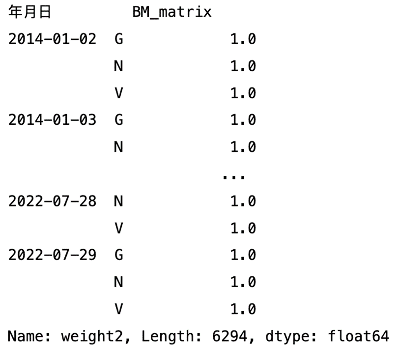
The return on the portfolio is calculated by subtracting the return on the growth stock portfolio from the return on the value stock portfolio to form a long-short portfolio, completing the HML factor.
df['return2'] = df['報酬率%']* df['weight2']
HML = df.groupby(['年月日','BM_matrix'])['return2'].sum()
HML.reset_index(inplace=True)
HML.set_index('年月日',drop=True, inplace=True)
HML = HML[HML['BM_matrix']=='V']['return2'] - HML[HML['BM_matrix']=='G']['return2']
HML.name = 'HML'
HML
Combine the calculated SMB and HML factors.
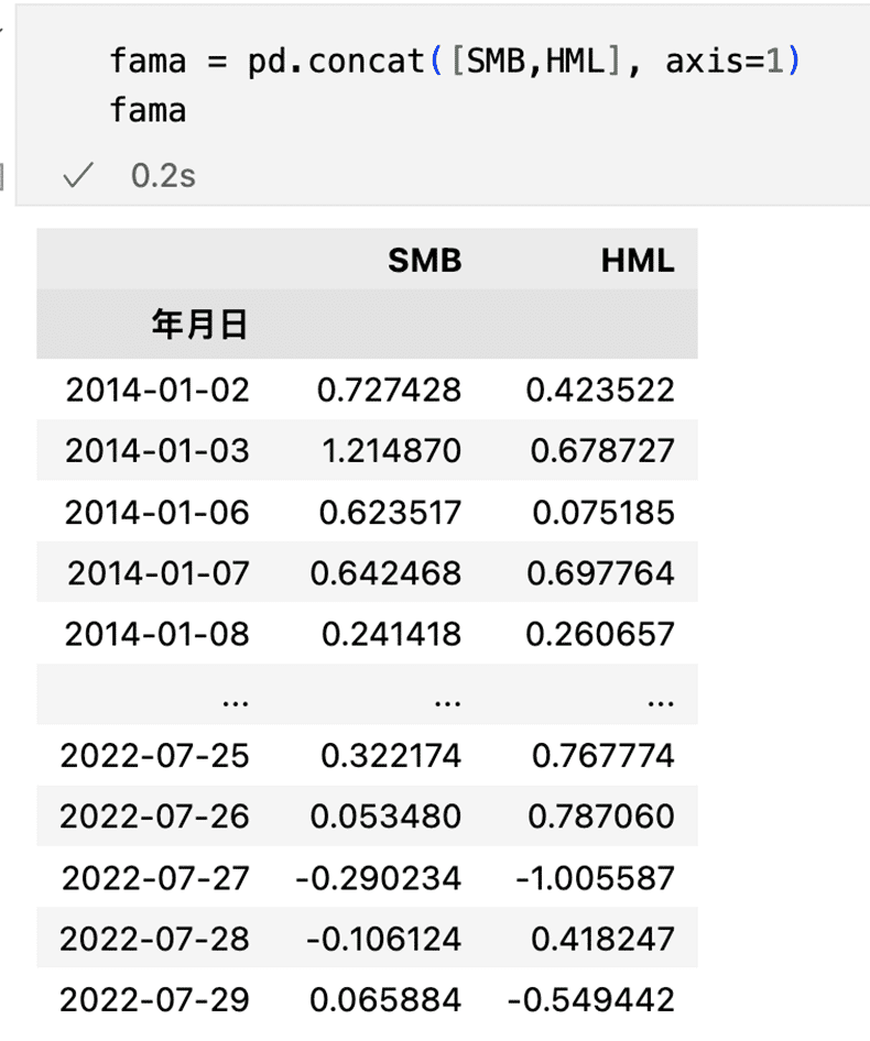
Combine the three factors into one table.
Y9999 = tejapi.get('TWN/APRCD1',  #從TEJ api撈取所需要的資料
                  chinese_column_name = True,
                  paginate = True,
                  mdate = {'gt':'2013-12-31', 'lt':'2022-07-01'},
                  coid='Y9999',
                  opts={'columns':['coid','mdate', 'roi']})
Screening out the return of individual stocks.
fama = fama.merge(Y9999[['年月日','報酬率%']], on='年月日')
fama.rename(columns = {'報酬率%':'rm'}, inplace=True)
fama.set_index('年月日',drop=True,inplace=True)
fama
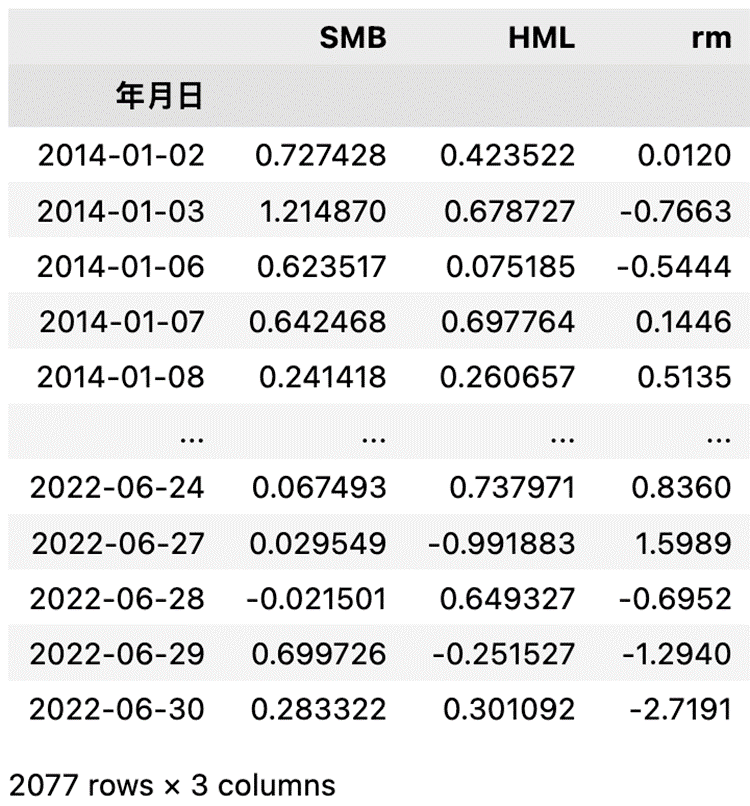
Screening out the return of individual stocks.
stock = df[['證券代碼', '年月日','報酬率%']]
stock.set_index('年月日', drop=True, inplace=True)
stock = stock.loc[:'2022-06-30']
stock
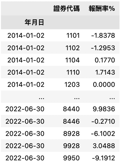
Our target portfolio is to combine a long-short strategy by deducting the alpha of the first 20% from the last 20% of all stocks, with equal weighted, and rebalancing by adjusting the portfolio every six months, using the data screened in the first six months for the second half of the year and backtesting.
m = pd.date_range('2013-12-31', '2022-07-31', freq='6M').to_list()
X = sm.add_constant(fama)
stock_list = stock['證券代碼'].unique()

b = pd.DataFrame()
for j in stock_list:
    a=[]
    for i in range(len(m)-1):
        try:
            Y = (stock[stock['證券代碼']== j]).loc[m[i]:m[i+1]]
            result = sm.OLS(Y['報酬率%'], X.loc[m[i]:m[i+1]]).fit()
            a.append(result.params[0])
        except:
            pass
    j = str(j)
    c = pd.DataFrame({'證券代碼':([j]*len(a)), 'alpha':a}, index=m[1:len(a)+1])
    b = pd.concat([b,c])
b.index.name = '年月日'
The alpha values of the 80th percentile and the 20th percentile are calculated, and stocks above the 80th percentile are screened out to form the long portfolio, while those below 20% form the short portfolio.
alpha1 = b.groupby('年月日')['alpha'].apply(lambda x : x.quantile(0.8))
alpha1.name = 'alpha0.8'
alpha2 = b.groupby('年月日')['alpha'].apply(lambda x : x.quantile(0.2))
alpha2.name = 'alpha0.2'
b = b.merge(alpha1, on='年月日')
b = b.merge(alpha2, on='年月日')
long = (b.where(b['alpha'] > b['alpha0.8'])).dropna()
short = (b.where(b['alpha'] < b['alpha0.2'])).dropna()
Do some data pre-processing before backtesting?
stock1 = df[['證券代碼','年月日','收盤價(元)']]
stock1.set_index('年月日',drop=True, inplace=True)
stock1 = stock1.loc[:"2022-06-30"]
stock1['證券代碼'] = stock1['證券代碼'].astype('str')
Calculate the return of the long portfolio and the return of the short portfolio, and calculate the return of this alpha strategy.
ret = []
for i in range(1, len(m)-1):
    qq = (stock1.loc[m[i]:m[i+1]])['證券代碼'].isin((long.loc[m[i]])['證券代碼'].tolist())
    a = ((stock1.loc[m[i]:m[i+1]])[qq]).groupby('證券代碼')['收盤價(元)'].tail(1).sum()
    b = ((stock1.loc[m[i]:m[i+1]])[qq]).groupby('證券代碼')['收盤價(元)'].head(1).sum()
    c = len((long.loc[m[i]])['證券代碼'].tolist())
    long_ret = ((a/b)-1)/c
    qq1 = (stock1.loc[m[i]:m[i+1]])['證券代碼'].isin((short.loc[m[i]])['證券代碼'].tolist())
    a1 = ((stock1.loc[m[i]:m[i+1]])[qq1]).groupby('證券代碼')['收盤價(元)'].tail(1).sum()
    b1 = ((stock1.loc[m[i]:m[i+1]])[qq1]).groupby('證券代碼')['收盤價(元)'].head(1).sum()
    c1 = len((short.loc[m[i]])['證券代碼'].tolist())
    short_ret = ((a1/b1)-1)/c1
    ret.append(long_ret - short_ret)
Theoretically, alpha represents the excess return, which can exceed that earned by the market, but from the results, we found that the return of the portfolio formed by using this strategy is between 0 and below, regardless of the general market ups and downs, which shows that these factors are already in doubt of failure.
y9999  = tejapi.get('TWN/APRCD1',  #從TEJ api撈取所需要的資料
                  chinese_column_name = True,
                  paginate = True,
                  mdate = {'gt':'2013-12-31', 'lt':'2022-07-01'},
                  coid='Y9999',
                  opts={'columns':['coid','mdate', 'close_adj']})

y9999.set_index('年月日' ,drop=True, inplace=True)

a = []
for i in range(1 , len(m)-1):
    b = (((y9999.loc[m[i]:m[i+1]]).tail(1)['收盤價(元)'].values / (y9999.loc[m[i]:m[i+1]]).head(1)['收盤價(元)'].values) -1)[0]
    a.append(b)

ret['大盤'] = a
ret[['ret', '大盤']].apply(lambda x :x*100)
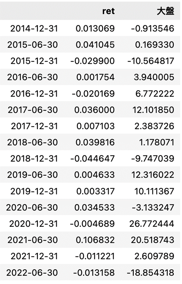
From the results, we can see that the return of our alpha-seeking portfolio is almost zero, probably because the Fama&French three-factor model was discovered early, and the abnormal return opportunities have already been discovered by investors, so it fails. Readers can learn more about other factor models, such as the five-factor model proposed by Fama & French in 2015, to test the performance in practice. Although the return of the three-factor model does not seem to be particularly good, it is still a very important part of asset pricing and is used by many in academia and the industry.
We will also introduce the use of the TEJ database to construct various indicators and backtest the performance of the indicators, welcome to purchase the plans offered in TEJ E-Shop and use the well-complete database to find the potential event.