Backtesting and stock-picking strategy with machine learning

Table of Contents
To put it simply, random forest is one of algorithms made up of many decision trees with the adoption of bagging and random sampling. Since it’s based on CART algorithm, it can handle both classification and continuous data. Other advantages such as its comparability with high dimensional data, high tolerance with noise, high accuracy of fitting results, so it’s commonly used in business competition like Kaggle.
In this article, we’ll treat financial data as features that are used to predict the movement of stock price, so it belongs to binary classification problem. Then see whether there’s valuable information gained from the fitted model to improve our stock-picking strategy.
Windows OS and Jupyter Notebook
#Basic function
import pandas as pd
import numpy as np
import matplotlib.pyplot as plt#Machine learning
from sklearn.ensemble import RandomForestClassifier#TEJ API
import tejapi
tejapi.ApiConfig.api_key = 'Your Key'
tejapi.ApiConfig.ignoretz = True
Step 1. Obtain industry code, financial and return data
security = tejapi.get('TWN/ANPRCSTD',
mkt = 'TSE',
stypenm = '普通股',
paginate = True,
chinese_column_name = True)#Store firms' codes
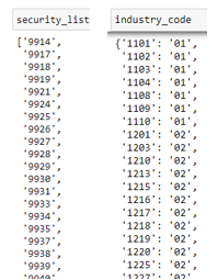
security_list = security['證券碼'].tolist()
#Store industries' codes
industry_code = security[['證券碼', 'TSE業別']]
industry_code = industry_code.set_index('證券碼').to_dict()['TSE業別']
First of all, obtain TSE-listed stocks’ codes and their corresponding industries’ codes. We save the latter one as a dictionary as shown below.
groups = []
while True:
    if len(security_list) >= 50:
        groups.append(security_list[:50])
        security_list = security_list[50:]
    elif 0 <= len(security_list) < 50:
        groups.append(security_list)
        break
Here we form several groups with 50 firms each group for the next step. Because if we obtain huge amount of data at one time, the failure may happen.
fin_data = pd.DataFrame() #Financial
ret_data = pd.DataFrame() #Return
date_data = pd.DataFrame() #Datefor group in groups:
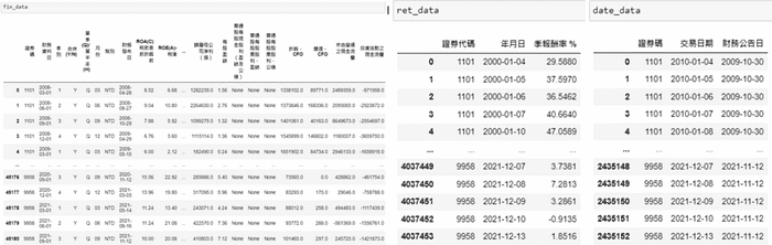
fin_data = fin_data.append(tejapi.get('TWN/EWIFINQ',
coid = group,
chinese_column_name = True,
paginate = True)).reset_index(drop=True)
ret_data = ret_data.append(tejapi.get('TWN/APRCD2',
coid = group,
opts = {'columns': ['coid', 'mdate', 'roi_q']},
paginate = True,
chinese_column_name = True)).reset_index(drop=True)
date_data = date_data.append(tejapi.get('TWN/EWFINDATE2',
coid = group,
opts = {'columns': ['coid', 'mdate', 'fin_date']},
paginate = True,
chinese_column_name = True)).reset_index(drop=True)
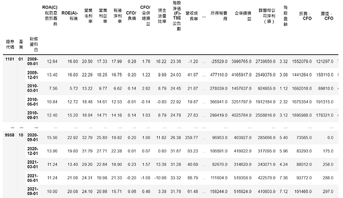
Then use the loop to get each groups’ financial and seasonal stock return data. It’s worth noting that the frequency of seasonal stock return is daily, because it’s the cumulative seasonal return before that date. It’s like a rolling stock return, thus it has data for each trading day. date_data is the table provided by TEJ, and it’s very useful while combining return and financial data.
Step 2. Merge data
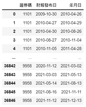
date_data = date_data.groupby(['證券碼', '財務公告日']).last().reset_index()
date_data = date_data.rename(columns = {'交易日期':'年月日', '財務公告日':'財報發布日'})
Obtain the last trading date before the next financial statement announcement date, because we’ll use this date to combine with the date of seasonal return. That’s to say, the seasonal return will represent the cumulative return after the financial statement announcement date. Finally, we change the column names to prepare for merging date.
merge = date_data.merge(fin_data, on = ['證券碼', '財報發布日'])
merge = merge.rename(columns = {'證券碼':'證券代碼'})
merge = merge.merge(ret_data, on = ['證券代碼', '年月日'])
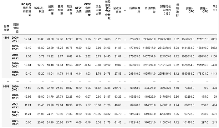
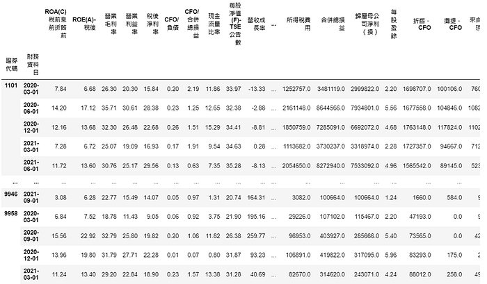
merge = merge.set_index(['證券代碼', '財務資料日']).select_dtypes(include=np.number)
Combine all the data and set codes of stock and date as our new indexes. Then only keep the numeric columns as features to predict the return movement.
Step 1. Split dataset into training and testing date and train the model
condition = merge.index.get_level_values('財務資料日') < '2020'
train_data = merge[condition].fillna(0)
test_data = merge[~condition].fillna(0)
rf = RandomForestClassifier(n_estimators=100, criterion= 'entropy')
rf.fit(train_data.drop(columns = '季報酬率 %'), train_data['季報酬率 %'] > 0)
The dataset before 2020 is used as training data and testing data otherwise. We fill the missing value with zero and finally fit the random forest model with features and boolean labels in training dataset.
Step 2. Model performance
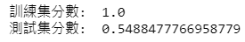
print("訓練集分數: " , rf.score(train_data.drop(columns = '季報酬率 %'), train_data['季報酬率 %'] > 0))
print("訓練集分數: " , rf.score(test_data.drop(columns = '季報酬率 %'), test_data['季報酬率 %'] > 0))
selected = rf.predict(test_data.drop(columns = '季報酬率 %'))
test_data[selected]
Use the predicted outcome as ways of filtering stocks. So we will have stocks that are predicted to perform well in the next season.
plt.rcParams['font.sans-serif'] = ['Microsoft JhengHei'] #顯示中文
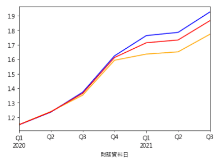
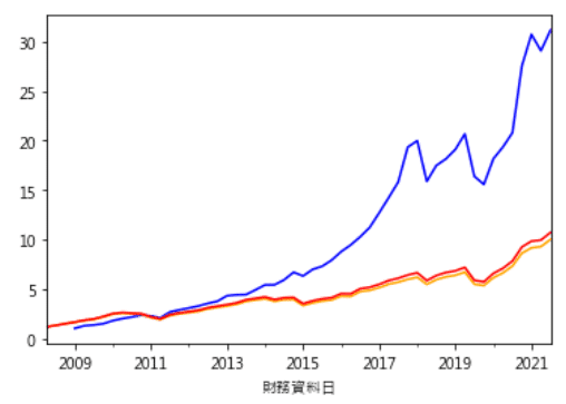
(test_data[selected].groupby('財務資料日').mean()['季報酬率 %']*0.01 + 1).cumprod().plot(color = 'blue') #randomforest
(test_data[~selected].groupby('財務資料日').mean()['季報酬率 %']*0.01 + 1).cumprod().plot(color = 'orange') #benchmark1
(test_data.groupby('財務資料日').mean()['季報酬率 %']*0.01 + 1).cumprod().plot(color = 'red') #benchmark2
We draw three lines here. Blue line means the cumulative return of portfolio based on model’s prediction. Orange line is the cumulative return of portfolio formed by selecting the stocks that are predicted to fall in stock return as our benchmark. Red line means we own all of the stocks without any filtering. It can be seen that blue line is the best of the three lines.
Step 1. Choose important features
feature_name = train_data.columns[:-1]
important = pd.Series(rf.feature_importances_, index = feature_name).sort_values(ascending=False)
important.head(20)
Observe the most 20 important features to be standards of selecting stocks
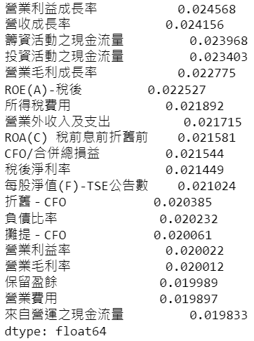
positive_features = ['營業利益成長率', '營收成長率', '投資活動之現金流量', '營業毛利成長率', 'ROE(A)-稅後', '營業外收入及支出', 'ROA(C) 稅前息前折舊前', 'CFO/合併總損益', '稅後淨利率', '每股淨值(F)-TSE公告數', '營業利益率', '營業毛利率', '來自營運之現金流量']
Next step is to subjectively choose the positive features, meaning the higher its value, the better the company is, from those 20 features. Since we will convert those values into percentiles and rank them by values, the higher value should signify it has better performance.
Step 2. The setting of same industry comparison
merge['產業'] = merge.index.get_level_values('證券代碼').map(industry_code)
merge = merge.reset_index().set_index(['證券代碼', '產業', '財務資料日'])
Here we map industry code, the value of the dictionary industry_code stored in data processing step, into a new column in merge. And set this column, security code and date as new index.
Step 3. Calculate important features scores to select stocks
score = merge[positive_features].groupby(['財務資料日', '產業']).rank(pct=True).sum(axis = 1)
rank = score.rank(pct = True)          #總分再rank
filters = rank > 0.97
(merge[filters].groupby('財務資料日').mean()['季報酬率 %']*0.01+1).cumprod().plot(color = 'blue')
(merge[~filters].groupby('財務資料日').mean()['季報酬率 %']*0.01+1).cumprod().plot(color = 'orange')
(merge.groupby('財務資料日').mean()['季報酬率 %']*0.01 + 1).cumprod().plot(color = 'red')
Then we group data by date and industry, and rank the values and convert them into percentiles in each group by using rank(pct=True) . Next is sum up the values horizontally and rank again. Finally we choose the data which is better than 97th percentiles of all data and backtesting. Following picture shows the cumulative return of this strategy (blue line) is superior than the other two benchmarks.
this_season = fin_data[fin_data['財務資料日'] == '2021-09-01']
this_season['產業'] = this_season['證券碼'].map(industry_code)
this_season = this_season.set_index(['證券碼', '財務資料日', '產業']).loc[:,positive_features]
score = this_season.groupby(['產業']).rank(pct=True).sum(axis = 1)
rank =  score.rank(pct = True)
firm_list = [i[0] for i in rank[rank > 0.97].index]
firms = tejapi.get('TWN/AIND',
                  coid = firm_list,
                  opts = {'columns':['coid','fnamec']},
                  paginate = True,
                  chinese_column_name = True)
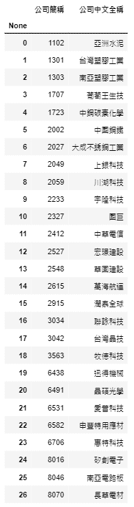
Choose the date equals to ‘2021–09–01’ , and also choose the best 3% of each industry. Then adopt database TWN/AIND to see the names of the companies
ret_sofar = tejapi.get('TWN/APRCD2',
coid = firm_list,
mdate = {'gte':'2021-09-30'},
opts = {'columns': ['coid', 'mdate', 'roia']},
paginate = True,
chinese_column_name = True)
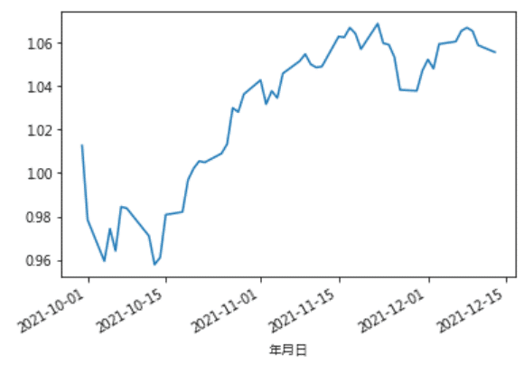
ret_sofar.groupby('年月日')['日報酬率 %'].mean().apply(lambda x: 0.01*x + 1).cumprod().plot()
The cumulative return of the newly-formed portfolio
Because TEJ API database has comprehensive and high quality data, it’s easier to handle in data processing step. We just need to merge the data, split the dataset and then we can start to build the model. Even though the accuracy is only 54.88%, we still can extract valuable information from the fitted model. Readers can try to adjust parameters while training the model, pick different combination of important features, use different databases or consider the trend of industries and do the second filtering. Lastly build the portfolio with optimal performance and see if its great performance will remain.
The content of this webpage is not an investment device and does not constitute any offer or solicitation to offer or recommendation of any investment product. It is for learning purposes only and does not take into account your individual needs, investment objectives and specific financial circumstances. Investment involves risk. Past performance is not indicative of future performance. Readers are requested to use their personal independent thinking skills to make investment decisions on their own. If losses are incurred due to relevant suggestions, it will not be involved with author.
