
Table of Contents
Survivorship bias refers to a type of error in research or observation where only the successful or surviving entities or events are considered, while the failures or disappearances are ignored or excluded. This bias can lead to a misunderstanding of the overall situation because observing only the successful or surviving entities may not represent the characteristics or true conditions of the entire population.
Survivorship bias often occurs in situations such as sample selection, study design, or retrospective analysis. A typical example is the research on aircraft defense reinforcement during World War II. Researchers primarily observed the damage to the aircraft that returned to base and then proposed defense recommendations based on these observations. However, this observation ignored the aircraft that were shot down and unable to return, leading to conclusions that may not apply to the entire group of aircraft.
Survivorship bias can also affect stock selection. During the stock selection process, investors tend to focus on stocks that perform well and generate profits while ignoring those that perform poorly or fail. This observation only considers examples of successful stocks, resulting in a bias in understanding the overall market or stock population.
Survivorship bias can lead investors to mistakenly believe that the outstanding stocks are representative or universally applicable and attribute their success to specific factors or strategies. Investors may be inclined to chase these successful stocks while overlooking market risks, industry trends, and other important stock selection factors. This exercise will use a simple trading strategy to illustrate the concept of survivorship bias.
This article uses Mac OS as a system and Jupyter Notebook as an editor.
import pandas as pd
import numpy as np
import tejapi

api_key = 'your_api_key'
tejapi.ApiConfig.api_key = api_key
tejapi.ApiConfig.ignoretz = TrueThe sampling period is from January 1, 2020, to December 31, 2022. Taking the biotechnology and healthcare companies as an example, stock price information was gathered as the analytical data.
comp_data = tejapi.get('TWN/ANPRCSTD',
                   paginate = True,
                  opts = {"columns":["coid", "mdate", "mkt", "stype", "list_date", "delis_date", "tseind"]}
                  )

#取得生技醫療類股代號,類別代碼為22
coid_lst = list(comp_data.loc[(comp_data["stype"] == "STOCK") & (comp_data["tseind"] == "22")]["coid"])

gte, lte = "2020-01-01", "2022-12-31"
price_data = tejapi.get('TWN/AAPRCDA',
                        paginate = True,
                        coid = coid_lst,
                        mdate = {"gte":gte, "lte":lte},
                        opts = {"columns":["coid", "mdate", "fld014", "cls60", "close_d"]}
)Securities Attribute Dataset displays the current status of the underlying securities, whether it is listed or delisted. On the other hand, Listed Adjusted Daily Stock Price Dataset — (mean) contains stock price for all companies that have been listed and delisted on the market.
price_data["coid"] = price_data["coid"].astype(str)
inter_coid = list(set(coid_lst).intersection(set(price_data["coid"].unique())))
price_data[price_data["coid"].isin(inter_coid)]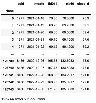
In this experiment, we will use the simplest moving average backtesting method, comparing the short-term moving average with the long-term moving average. When the short-term moving average break through the long-term moving average, it is known as a “Golden Cross” and is considered as a buy signal. Conversely, when the short-term moving average falls below the long-term moving average, it is referred to as a “Death Cross” and is considered a sell signal. For ease of calculation, this trading strategy only trades one unit of stock whenever a trading signal is triggered unless it is the last day of the target price information, in which case the position will be closed. In this exercise, we will use a 10-day moving average as the short-term moving average and a 60-day moving average as the long-term moving average.
First, we will group the stock price data according to the stock symbols.
fltr_price_data = price_data[price_data["coid"].isin(inter_coid)]
group = fltr_price_data.groupby("coid")
Next, we will define the function for the moving average trading strategy. This function will ultimately return two pieces of data. First, it will provide a data table of the trading history, which includes the trading date, stock symbol, buy/sell indication, trade price, trade units, remaining cash, and position holdings. Second, it will provide the remaining cash balance after the completion of all trades.
def MA_strategy(df, principal):
    position = 0
    lst = []

    for i in range(len(df)):
        if df["fld014"].iloc[i] > df["cls60"].iloc[i] and principal >= float(df["close_d"].iloc[i])*1*1000:
            principal -= float(df["close_d"].iloc[i])*1*1000
            position += 1
            lst.append({
                "日期": df["mdate"].iloc[i],
                "標的": df["coid"].iloc[i],
                "買入/賣出": "買入",
                "單價": float(df["close_d"].iloc[i]),
                "單位": 1,
                "剩餘現金": principal,
                "部位" : position
            })

        elif df["fld014"].iloc[i] < df["cls60"].iloc[i] and position > 0:
            principal += float(df["close_d"].iloc[i])*1*1000
            position -= 1

            lst.append({
                "日期": df["mdate"].iloc[i],
                "標的": df["coid"].iloc[i],
                "買入/賣出": "賣出",
                "單價": float(df["close_d"].iloc[i]),
                "單位": 1,
                "剩餘現金": principal,
                "部位" : position
            })

        elif i == len(df)-1 and position > 0:
            principal += float(df["close_d"].iloc[i])*position*1000
            position -= position
            lst.append({
                "日期": df["mdate"].iloc[i],
                "標的": df["coid"].iloc[i],
                "買入/賣出": "賣出",
                "單價": float(df["close_d"].iloc[i]),
                "單位": position,
                "剩餘現金": principal,
                "部位" : position
            })

    df_output = pd.DataFrame(lst)

    return (df_output, principal)
Since the main objective of this exercise is to demonstrate the presence of survivorship bias in the stock market, the trading strategy in this case does not focus on completely realistic operations and allocations. Instead, the entire trading strategy is treated as an independent variable, the portfolio configuration is treated as a control variable, and the reflected investment returns are treated as the dependent variable. Here, we assume that each stock has the same initial capital, which is set at 1 million dollars.
We will consider all healthcare and biotechnology companies that were listed or listed on the market at any time point between January 1, 2020, and December 31, 2022, as the investment portfolio.
print(f'2020–01–01 至 2022–12–31狀態曾經為上市櫃的公司數量:{len(list(comp_data.loc[(comp_data["coid"].isin(inter_coid))]["coid"]))}')
principal = 1000000
total_return_1 = 0
df = pd.DataFrame(columns = ["日期", "標的", "買入/賣出", "單價", "單位", "剩餘現金", "部位"])

for g in group.groups.keys():
    reuslt = MA_strategy(group.get_group(g), principal)
    total_return_1 += round(reuslt[1], 2)
    df = pd.concat([df, reuslt[0]], ignore_index=True)
Next, we will calculate the ROI (Return on Investment) by summing up the final remaining cash amount for each stock and dividing it by the initial amount, which is 1 million multiplied by the number of stocks in the portfolio.
total_return = (total_return_1/(1000000*len(group.groups.keys())) - 1) *100
print(f"ROI : {total_return}%")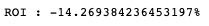
The calculated overall performance is -14%. Next, we will exclude nine companies that were delisted between January 1, 2020, and December 31, 2022. In the Securities Attribute Dataset, the column “mkt” represents the market status, and if it is “DIST,” it indicates that the company is currently delisted. We will use this as the basis for filtering the data.
Following the previous steps, we will group the filtered stock price data based on the stock symbols.
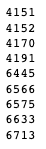
without_dist_coid = comp_data.loc[(comp_data["coid"].isin(inter_coid)) & (comp_data["mkt"] != "DIST")]["coid"].unique()
fltr_price_data = price_data[price_data["coid"].isin(without_dist_coid)]
group = fltr_price_data.groupby("coid")
Next, we will execute the trading strategy as before.
principal = 1000000
total_return_2 = 0
df_without_dist = pd.DataFrame(columns = ["日期", "標的", "買入/賣出", "單價", "單位", "剩餘現金", "部位"])
for g in group.groups.keys():
    reuslt = MA_strategy(group.get_group(g), principal)
    total_return_2 += round(reuslt[1], 2)
    df = pd.concat([df_without_dist, reuslt[0]], ignore_index=True)
return_without_dist = (total_return_2/(1000000*len(group.groups.keys())) - 1) *100
print(f"ROI : {return_without_dist}%")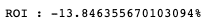
According to the calculations, the performance after excluding delisted companies is indeed slightly better compared to the original performance. Although both performances are negative, we can clearly observe the difference in returns through the program implementation.
Typically, when conducting performance backtesting, investors tend to select companies that survived within the sampling period and overlook the inclusion of delisted companies during the testing period. The surviving companies are objectively considered to have better fundamentals, resulting in better investment returns for the model. However, such results are not accurate or comprehensive as the inclusion of delisted company stock price information is necessary for a more accurate reflection of the market conditions at that time.
Survivorship bias can lead to the over-optimization of stock selection strategies. If investors only base their stock selection on specific factors of past successful stocks and ignore the overall market changes and uncertainties, they may fail to adapt to market fluctuations, thus affecting investment outcomes. To avoid the negative impact of survivorship bias on stock selection, investors should adopt a comprehensive research approach that includes considering both successful and unsuccessful stocks. They should focus on factors such as overall market trends, industry developments, company fundamentals, and risk management, rather than relying solely on the performance of past successful stocks. Additionally, investors should have a long-term investment perspective, avoid excessive focus on short-term stock performance, and establish their own investment strategies that align with their individual investment goals and risk tolerance.
Please note that this strategy and the mentioned stocks are for reference purposes only and do not constitute any commodity or investment advice. We will also introduce the use of the TEJ database to construct various indicators and backtest their performance. Therefore, readers who are interested in various trading backtests are welcome to purchase related packages from the TEJ E-Shop, using high-quality databases to build their own suitable trading strategies.
