
Most investors mainly do their investment from the technical analysis, the fundamental analysis and the chip analysis. The technical analysis will use a lot of historical data among these 3 methods. Therefore, we are going to use Python to share some technical analysis indicators which investors used frequently this week.
Table of Contents
The technical analysis mainly uses past information such as historical data to explain the trends or determining the timing of investment. However, the past is the past. But when you want to have a quantitative understanding of the current market situations, technical analysis can provide some indicators for investors to simplify the past information for them to reference.
We are not going to compare the pros and cons of the technical analysis in this article. How to use codes to have a further understanding of the commonly used technical indicators is the main goal this time!
Example of TA:Moving Average, KD Indicators, RSI, MACD, etc.Before we start the introduction, let’s get the data for our TEJ API first! We are going to use the historical data of UMC(2303) this time.
import tejapi
import pandas as pd
import numpy as np
import datetime
tejapi.ApiConfig.api_key = "your key"
UMC = tejapi.get(
    'TWN/EWPRCD',
    coid = '2303',
    mdate={'gte':'2020-04-01', 'lte':'2021-04-25'},
    opts={'columns': ['mdate','open_d','high_d','low_d','close_d',              'volume']},
    paginate=True)
UMC = UMC.set_index('mdate')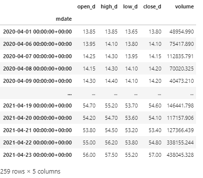
After getting the historical data, now we can enter our next step!
MACD compares the exponential moving average(EMA) of long(26) and short(12) days, subtracts to find the difference(DIF), and then calculates the difference again on the EMA. To put it simply, MACD is used to judge the trading timing of the target through the staggered condition between the EMA of long and short days.
EMA: The difference between the simple moving average is that EMA places a greater weight and significance on the most recent data points.
DIF(Short-term): The subtraction of short-term and long-term EMA, which usually represents a short-term trend.
MACD(Long-term): Taking the EMA of DIF again, which usually can judge the long-term trend.
def MACD(DF, a = 12, b =26, c =9):
    '''
    SMA: rolling
    EMA: ewm
    '''
    df = DF.copy()
    df["EMA_Fast"] =
         df['open_d'].ewm(span = a, min_periods = a).mean()
    df["EMA_Slow"] =
         df['open_d'].ewm(span = b, min_periods = b).mean()
    df["DIF"] = df["EMA_Fast"] - df["EMA_Slow"]
    df["MACD"] = df['MACD'].ewm(span = c, min_periods = c).mean()

    return df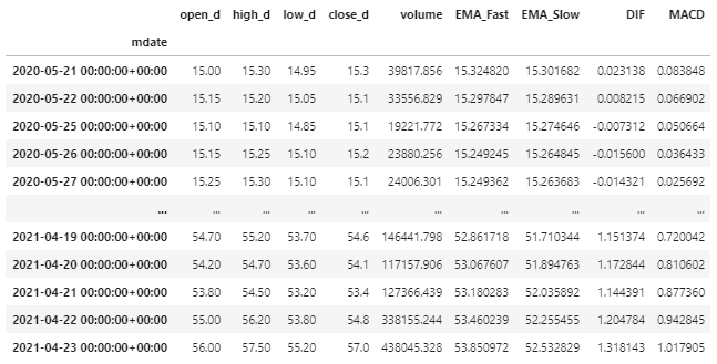
The Bollinger Bands are made by the combination of 3 lines, which are the simple moving average, the upper standard deviation line, and the lower standard deviation line to show the safe area of the stock price.
The reason for using 2 standard deviations is that in the statistical normal distribution, there is a 95% probability that it will fall between the 2 standard deviations. Although the market may not completely follow the normal distribution, it will still fall between 2 standard deviations most of the time.
def BollingerBand(DF, n=20):
    '''
    Standard Deviation: std
    '''
    df = DF.copy()
    df['SMA'] = df['close_d'].rolling(window = n).mean()
    df['BB_20dstd_up'] =
         df['SMA'] + 2*df['close_d'].rolling(window = n).std(ddof=0)
    df['BB_20dstd_down'] =
         df['SMA'] - 2*df['close_d'].rolling(window = n).std(ddof=0)
    df['BB_width'] = df['BB_20dstd_up'] - df['BB_20dstd_down']
    df.dropna(inplace = True)

    return df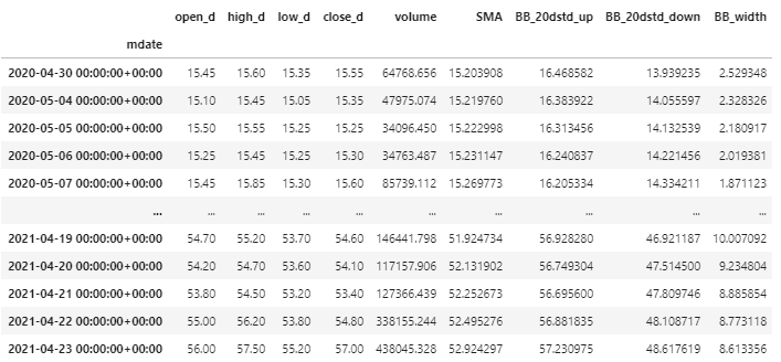
The Relative Strength Index is mainly used to access the “strength of the buyer’s and seller’s strength” in the stock market, and to access the overbought/oversold situation through the recent price changes. The value of RSI is within 0 to 100. The larger or smaller the value, the stronger the strength. Usually, below 30 means oversold, over 70 means overbought.
def RSI(DF, n=14):
    '''
    n-day avarage increase = sum of n-day total daily increase ÷ n
    n-day avarage decrease = sum of n-day total daily decrease ÷ n
    '''
    df = DF.copy()
    df['daliy_change'] =
         df['close_d'] - df['close_d'].shift(1)
    df['dUp'] =
         np.where(df['daliy_change'] >= 0, df['daliy_change'], 0)
    df['dDown'] =
         np.where(df['daliy_change'] < 0, -df['daliy_change'], 0)
avg_dUp = []
    avg_dDown = []
    dUp = df['dUp'].tolist()
    dDown = df['dDown'].tolist()

    for i in range(len(df)):
        if i < n:
            avg_dUp.append(0)
            avg_dDown.append(0)
        elif i == n:
            avg_dUp.append(df['dUp'].ewm(span = n).mean()[n])
            avg_dDown.append(df['dDown'].ewm(span = n).mean()[n])
        else:
            avg_dUp.append(((n-1)*avg_dUp[i-1] + dUp[i])/n)
            avg_dDown.append(((n-1)*avg_dDown[i-1] + dDown[i])/n)

    df['avg_dUp'] = np.array(avg_dUp)
    df['avg_dDown'] = np.array(avg_dDown)
df['RS'] = df['avg_dUp']/df['avg_dDown']
    df['RSI'] = df['RS'].apply(lambda x: x/(1+x) * 100)

    return df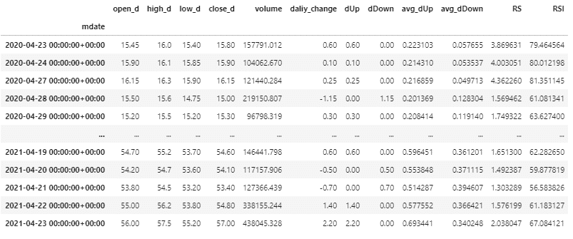
ATR refers to the true range of the stock price fluctuations within a period of time(14 days used in this article), which is a measure of the volatility of the target.
In order to calculate the ATR, we must first calculate the TR, and the TR refers to the largest number among the following 3 numbers:
1. H-L: Today’s high minus today’s low.
2. H-PC: The absolute value of today’s high minus yesterday’s close.
3. L-PC: The absolute value of today’s low minus yesterday’s close.
def ATR(DF, n=14):
    '''
    Close Price of Previous Day: close.shift()
    '''
    df = DF.copy()
    df['H-L'] = abs(df['high_d'] - df['low_d'])
    df['H-PC'] = abs(df['high_d'] - df['close_d'].shift())
    df['L-PC'] = abs(df['low_d'] - df['close_d'].shift())
    df['TR'] = df[['H-L', 'H-PC', 'L-PC']].max(axis =1, skipna =False)
    df['ATR'] = df['TR'].ewm(span =n, min_periods=n).mean()

    return df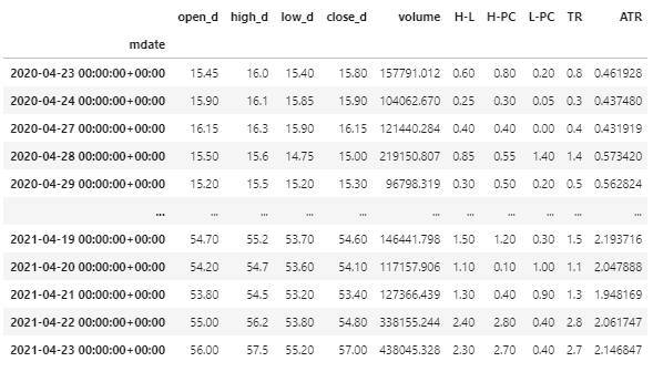
The KD Indicator is mainly used to show the trend of the asset’s price in the past period of time. The 2 values of K and D are used to find possible price turning points as trading signals. The concept of the KD indicator is similar to RSI, but the difference is that the KD indicator is based on the relative high or low of the latest price, while the RSI comparing the ratio of the strength of the buy/sell.
Calculation:
RSV: (Today’s close -14day LOW)/(14day High -14day Low) * 100
K: Yesterday’s K*(2/3)+Today’s RSV*(1/3)
D: Yesterday’s D*(2/3)+Today’s K*(1/3)
def KD(DF, n = 14):
    '''
    function to calculate KD
    '''
    df = DF.copy()
    df['High_9D'] = df['high_d'].rolling(n).max()
    df['Low_9D'] = df['low_d'].rolling(n).min()
    df['RSV'] =
        (df['close_d'] - df['Low_9D']) / (df['High_9D'] - df['Low_9D']) * 100
df = df.dropna()
    df['K'] = np.zeros(len(df))
    df['D'] = np.zeros(len(df))

    for i in range(len(df)):
        if i == 0:
            df['K'][i] = 50
            df['D'][i] = 50
        else:
            df['K'][i] = df['K'][i-1]*(2/3) + df['RSV'][i]*(1/3)
            df['D'][i] = df['D'][i-1]*(2/3) + df['K'][i]*(1/3)

    return df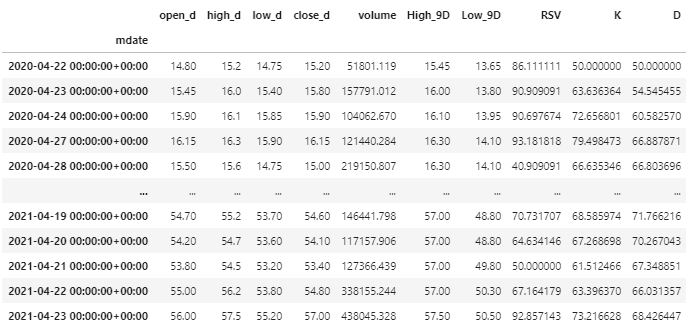
We are going to use some indicators we’ve mentioned above to construct our strategy. Notice!! The signals are built without serious testing. The purpose is only to introduce how to applicate those indicators, so even if the results are not bad, you shouldn’t use them directly!!
print("Calculating returns for ","UMC")
ret = []
for i in range(1,len(UMC)):
    buy_signal = UMC["DIF"][i]> UMC["MACD"][i] and \
                 UMC["K"][i]> 70 and \
                 UMC["K"][i] > UMC["K"][i-1]
sell_signal =
     UMC["low_d"][i] < UMC["close_d"][i-1] - UMC["ATR"][i-1]
if tickers_signal["UMC"] == "":
        tickers_ret["UMC"].append(0)
        if buy_signal:
            tickers_signal["UMC"] = "Buy"
elif tickers_signal["UMC"] == "Buy":
        if sell_signal:
            tickers_signal["UMC"] = ""
            tickers_ret["UMC"].append(
    ((UMC["close_d"][i] - UMC["close_d"][i-1])/UMC["close_d"][i-1]))
        else:
            tickers_ret["UMC"].append(
      (UMC["close_d"][i]/UMC["close_d"][i-1])-1)
UMC['ret'] = np.array(tickers_ret["UMC"])
After finding the signal points and the rate of return, let’s make a simple plot to see how this strategy performs!
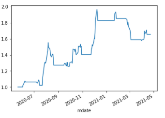
It seems that our performance is acceptable, but we have ignored many possible costs of course. However, we could understand that if we use the technical analysis indicators properly, investors can indeed simplify a lot of past information and find the trading signals.
Different people will have different opinions toward the same data, but the indicators created from the data could still be used as a tool for investors to judge whether to buy or sell. This article is to share how to build these indicators through Python by yourself. Of course, there are many packages that have included these indicators, but through these processes, you will understand more about these indicators and can adjust the parameters by yourself in the future!💪💪
If you like this topic, please click 👏 below, giving us more support and encouragement. Additionally, if you have any questions or suggestions, please leave a message or email us, we will try our best to reply to you.👍👍