
Using Python to fulfill the investing strategy of Benjamin Graham meanwhile backtesting it in the Taiwan stock market.
Table of Contents
We will introduce the defensive investing strategy which was created by Benjamin Graham — master of value investing. Benjamin Graham is the recognized pioneer of securities analysis. His first private fund was founded in 1923, and its performance was very good in its first shot. In 1925, it was liquidated and dissolved due to the disagreement of the partners. In 1926, he established Graham Joint Account, a joint venture, with his friend By the beginning of 1929, the capital scale had grown from $450,000 to $2.5 million (non-new investors). Overnight, Graham’s name became the darling of Wall Street. The owners of many listed companies hoped that Graham could be responsible for their funds, but they all were rejected because Graham believed that the stock market had soared excessively.
In 1934, Graham and David L. Dodd co-authored the book “Security Analysis”, which became the first ancestors of securities analysis. Before Graham, securities analysis could not be regarded as a science. This book is still one of the textbooks in teaching securities analysis for universities.
Contemporary well-known fund managers such as Warren Buffett, John Neff, Tom Knapp, et al., are Graham’s students. Therefore, as long as fund managers on Wall Street who used Value Investing, we can say that they are all Graham’s disciples.
1. Select the companies whose yearly revenue is more than 100 million, or whose yearly revenue is more than 50 million for public utilities.
2. Liquid ratio is higher than 200% and the long-term liabilities do not exceed net current assets.
3. Select the companies which have earnings every year over the past 10 years.
4. Select the companies that have paid cash dividends every year over the past 20 years.
5. Select the companies whose 3-year average EPS has grown at least 1/3 over the past 10 years.
6. Stock price ÷ 3-year average EPS <15
7. Price to book values <1.5
8. The portfolio contains 10–13 stocks.
⬇️For the change in time and location, we adjusted to the above conditions.⬇️
1. Select the companies whose yearly revenue is more than the yearly average revenue of all listed companies.
2. Select the companies that have earnings every year over the past 5 years.
3. Select the companies that have paid cash dividends every year over the past 2 years.
4. Liquid ratio is higher than 200%.
5. Net current assets – long-term liabilities > 0
6. The absolute value of (recent 3-year average of net income -a recent 5-year average of net income)/recent 5-year average of net income > 0.33
7. PER1(calculated by the most recent 3-year average of EPS) ≤ recent 3-year average of PER.
8. PER(calculated by the sum of recent 4-quarter EPS)PBR ≤ recent 3-year average of PER*PBR.
Yearly revenue, Earnings, Cash Dividends, Liquid Ratio, Net Current Assets, Long-term Liabilities, average of Net Income, EPS, PBR
To construct the master strategy, we need to select all the variables which the strategy needs, so that we can calculate and combine them into one table for the following backtesting.
-IFRS Consolidated Simplified Statements (Cumulative)
-All Industries (TWN/AIM1A), Listed (OTC) Stock Price Returns (Daily)
-Rate of Return (TWN/APRCD2), Listed (OTC) Unadjusted Stock Prices (Yearly) (TWN/APRCY)
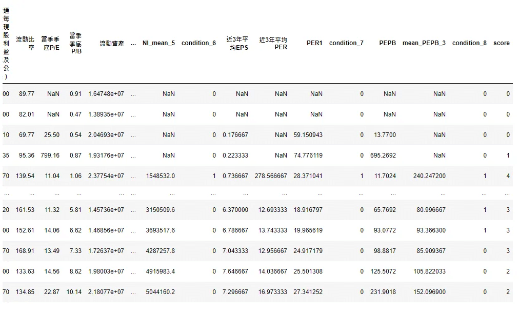
We use the score to sort the data and separate the data into five portfolios by quintiles, then we will backtest the performance of five portfolios respectively. For example, the top 20% of the score will be the first group, and 21% to 40% will become the second group……

date: Financial report date
buy_date: Assume 12/13 is T, then buy date is T+90.
sell_date: Sell date is buy_date+365.(holding period 1 year)
pf_H: Storing stock code of each portfolio.
data: Extracting yearly return of multi-stocks(pf_H), and the date set between buy_date and sell_date.
q1_ret: yearly return of multi-stocks(pf_H)
tw0050: Extracting yearly return of 台灣50指數(TRI50), and the date set between buy_date and sell_date.
The number of stock in portfolio: len(pf_H)
(including transition fee and tax).
weight : w = 1/len(pf_H)
weighted-average return: sum(w*q1_ret)
transition fee + tax : (0.1425*2*len(pf_H) + 0.3*1)
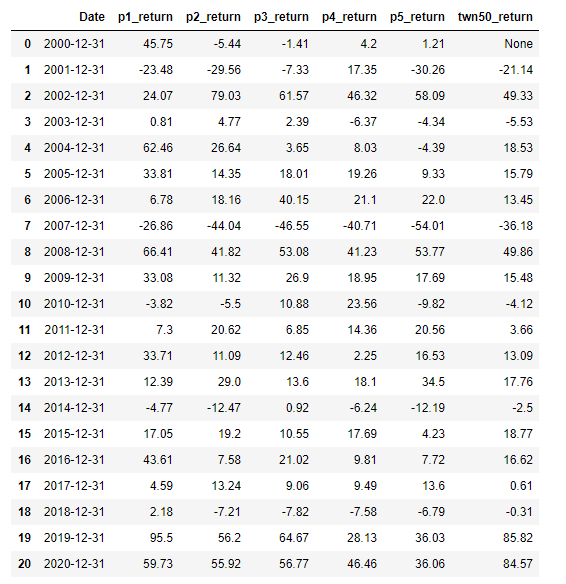
Taiwan 50 index was published after 2002, so we could not get the cumulative return in 2000.
Because the holding period is 1 year, the most recent data is the report of 2020Q4. Therefore, the buy date is 2021–03–31 and we will hold it till 2022–03–31. However, 2022–03–31 is in the future, so we can’t get the close price at that date now. Therefore, we have to kick out the return calculated in 2020Q4.
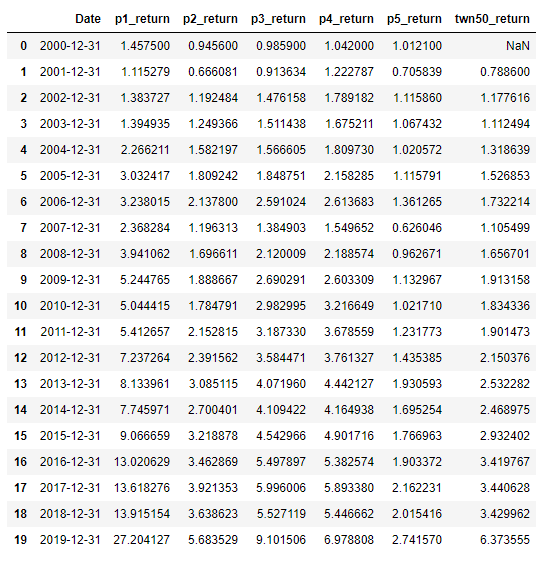
we explicitly mark TRI50 and each portfolio’s cumulative return with a different color.
plt.style.use('seaborn')
plt.figure(figsize=(10,5))
plt.xticks(rotation = 90)
plt.title('master invest strategy',fontsize = 20)
date = cum_ret['Date']
plt.plot(date,cum_ret.p1_return,color ='red',label='p1_return')
plt.plot(date,cum_ret.p2_return,color ='orange',label='p2_return')
plt.plot(date,cum_ret.p3_return,color ='blue',label='p3_return')
plt.plot(date,cum_ret.p4_return,color ='purple',label='p4_return')
plt.plot(date,cum_ret.p5_return,color ='green',label='p5_return')
plt.plot(date,cum_ret.twn50_return,color = 'black',label='twn50_return')
plt.legend(fontsize = 15)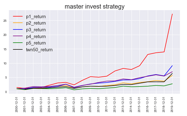
The result shows that the cumulative return of the highest score group (P1) is outperformed others, which is nearly 5 times higher than the benchmark — Taiwan 50 index(black line).
We further assess TRI50’s and five portfolios’ performance with Internal Rate of Return, Annualized Standard Deviation, sharp ratio, and max drawdown(%).

As we went deep into the performance calculations, the result shows that the annual return, Sharpe ratio, and max drop-down of the highest-score group (P1) all beat others, but it also has the highest volatility among others.
stk_ranking = result[result['財報年月']== '2020-12-01'].sort_values(by='score',ascending=False).reset_index(drop=True)
first_group = round(len(stk_ranking)*(0.2))
stk_ranking = stk_ranking.loc[0:first_group]['公司代碼'].tolist()
# 回台灣 50成分股查詢 P1組合的名稱
stk_info['stk_num'] = stk_info['成份股'].apply(lambda x: str(x).split(' ')[0])
stk_info['stk_cname'] = stk_info['成份股'].apply(lambda x: str(x).split(' ')[1])
stk_info['成份股'][stk_info['stk_num'].isin(stk_ranking)].to_list()
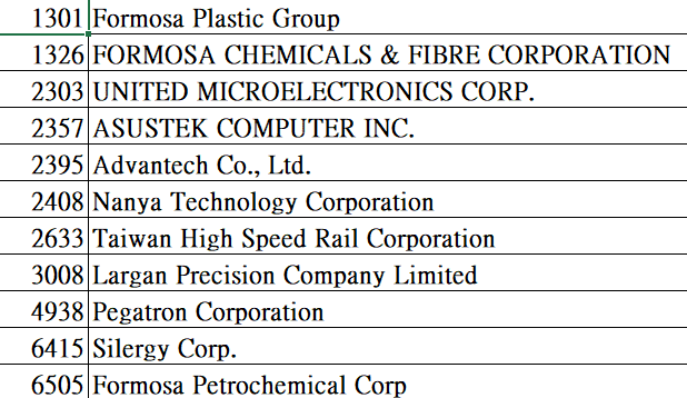
In this article, we use Python to fulfill the investing strategy of Benjamin Graham meanwhile backtesting it in the Taiwan stock market and further display the result of the strategy by table and plots. After seeing the result, isn’t it very impressive? According to the results of our backtest, if we have started to invest in the highest-scoring group since 2000, its cumulative return will exceed 20 times.
Via TEJ’s financial database, we can readily get every parameter required for the master strategy. Still, TEJ’s comprehensive database even contains data that can assist one in assessing the performance of the top 50 enterprises in Taiwan.
To make successful backtesting, we still need to pay attention to things such as the data quality, the length of data, whether there are bugs in your program, whether too many transaction costs are ignored, etc. As long as there is a mistake in these problems, it will distort the backtesting and lose money! Therefore, we have to pay attention to our backtesting results every time.
This study employed TEJ API data and utilized Python to construct various indicators and back-test their performance. For the complete code and details on the database project, please refer to the link below.
TEJ Quantitative datasets allow decision makers to get access to accurate data in real-time and improve strategy performance:
• Avoid look-ahead bias and reduce inaccurate assumptions
• Finding effective factors that facilitate quantitative modeling
Assess to databank