
Fulfill the investing strategy of Trinity Investment Management through python.
Table of Contents
Trinity Investment Management, founded in 1974, was only provided investment research advice for investment institutional clients, and it has managed investment portfolios for clients since 1980. In 1999, it became a member of Oppenheimer Funds, Inc., one of the largest mutual fund and investment management groups in the United States.
By the end of the first quarter of 2000, Trinity Investment Management has managed a total of US$4.2 billion for clients. Its investment philosophy was value-oriented and believed that the establishment of a successful value-based investment portfolio only requires simple and simplified concepts and systematic design. However, most fund managers didn’t accept it.
According to years of research conducted by Trinity Investment Management, the three elements of P/E ratio, P/B ratio, and dividend yield are combined to build an investment portfolio. During the 15 years from 1980 to 1994, the average annual return on investment reached 20.1% and beat the S&P 500 index by 6.8% every year. Stanford Calderwood, President of Trinity Investment Management, particularly emphasized the importance of dividend income to value investors and believed that the predictive data used by growth fund managers had no effect on the performance of the investment portfolio value.
This article might be hard to totally understand. However, don’t worry about it because we have provided you with the full source code and contact information at the bottom of the article. If you have any problems while this article, please leave a message below or email us!
According to the research of Trinity Investment Management, there are three results:
1. From 1980 to 1994, the 30% stocks in the S&P500 with the lowest P/E ratio were used as the portfolio (updated and replaced every quarter), and the average annual return was 17.5%, while the return of the S&P500 index during the same period was 13.3%.
2. At the same period, the 30% stocks in the S&P500 with the lowest P/B ratio were used as the portfolio (updated and replaced every quarter), and the average annual return was 18.1%, which was 4.8% higher than the S&P500 index return.
3. Take the 30% stocks in the S&P500 with the highest dividend yield as the investment portfolio, and the average annual return was 18.3%, which is 5% higher than the return of the S&P500 index.
1. Sort the companies’ daily P/E ratio from low to high, and select the lowest 30% of companies.
2. Sort the companies’ daily P/B ratio from low to high, and select the lowest 30% of companies.
3. Sort the companies’ daily dividend yield from high to low, and select the highest 30% of companies.
4. Finally, we take the union of these three conditions. The reason why we do not take the intersection is that companies with low P/E and P/B ratios but with high dividend yields are likely to have long-term business growth problems, and high dividend rates may be a cover for long-term stock prices that may fall below market expectations.
import tejapi
import pandas as pd
import numpy as np
tejapi.ApiConfig.api_key = "your key"
tejapi.ApiConfig.ignoretz = True
import datetime
import matplotlib.pyplot as plt
from datetime import datetime, timedelta
from functools import reduceFirst, we could get constitute stocks of Taiwan 50 index from TW50.csv. However, the format of constitute stocks contains both numbers and characters(Ex: 1101 台泥), so we could use the second line of code to help us get the numbers only.
Next, we could get financial data and stock price data through the TWN/AIM1A and TWN/APRCM databases respectively, and replace the daily data with quarterly data through the resample function in pandas.
stk_info = pd.read_csv('TW50.csv',engine='python')
stk_nums = stk_info['成份股'].apply(lambda x: str(x).split(' ')[0])
strategy_cols = ['公司代碼','財報年月','當季季底P/E', '當季季底P/B', '股利殖利率']
## 2008 to 2020
# Getting data
df_foundamental = pd.DataFrame()
q_df_stock = pd.DataFrame()
df_stock_Qrt = pd.DataFrame()
for stk in stk_nums:
df_foundamental = df_foundamental.append(tejapi.get('TWN/AIM1A'
,coid=stk
,mdate={'gte':'2008-01-01', 'lte':'2020-12-31'}
,paginate=True,chinese_column_name=True
,opts={'pivot':True}
)).reset_index(drop=True)
df_stock = tejapi.get('TWN/APRCM'
,coid=stk
,mdate={'gte':'2008-01-01', 'lte':'2020-12-31'}
,paginate=True,chinese_column_name=True)
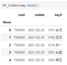
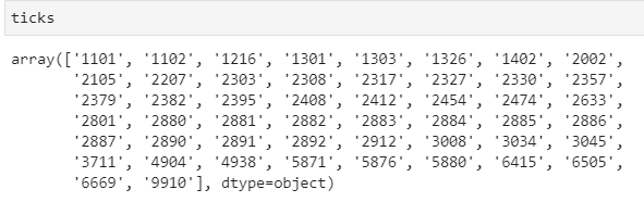
q_df_stock = q_df_stock.append(df_stock.resample('Q', on='年月').last().reset_index(drop=True))In addition to using TW50.csv here, we provide another method for you to select the 0050 constituent stocks. Through the TWN/AIDXS database, we can directly find the constituent stocks of 0050 at the specific time period, and ticks can be found in this method.
df_indexcomp = tejapi.get('TWN/AIDXS', coid= 'TWN50',
                  opts={'columns':['coid', 'mdate', 'key3']},
        mdate='gte':'2021/02/25','lte':'2021/02/25'},paginate=True)df_indexcomp['stk'] =
     [df_indexcomp.iloc[i,2].split(' ')[0] for i in range(df_indexcomp.shape[0])]df_indexcomp['name'] =
         [df_indexcomp.iloc[i,2].split(' ')[1] for i in range(df_indexcomp.shape[0])]ticks = df_indexcomp.stk.unique()
Next, because we want to merge the two data tables, we need to rename the columns in the two tables, select the data we want, and use the merge function in pandas to merge.
##financial report table
df_foundamental.rename(columns={'公司代碼':'coid','財報年月':'日期'},inplace=True)
df_foundamental = df_foundamental[['coid','日期','當季季底P/E', '當季季底P/B', '股利殖利率']]
##stock price table
q_df_stock.rename(columns={'證券代碼':'coid','年月':'日期'},inplace=True)
q_df_stock = q_df_stock[['coid','日期','收盤價(元)_月']]
##merge
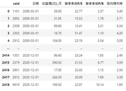
new_df = pd.merge(q_df_stock, df_foundamental, on = ['日期', 'coid'])
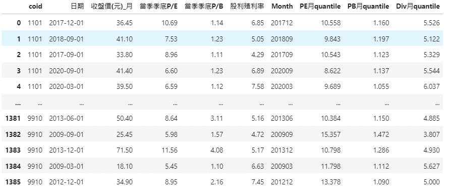
new_df.sort_values(by='日期').reset_index(drop=True)Then, you can see the following data table, the quarterly data of 0050 constituent stocks from 2008 to 2020, and quarterly PE, PB ratios, and dividend yield.
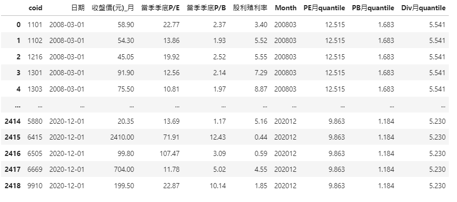
Since we will need three main conditions here, namely the P/E, P/B ratios, and the dividend yield. Therefore, we will first change the data format from the original 2008–03– 01 to 200803, and use the groupby function in pandas to compare all the same 200803 together, and then present our filtering conditions.
##data format change
new_df['日期'] = pd.to_datetime(new_df['日期'])
new_df['Month'] = new_df['日期'].apply(lambda x:datetime.strftime(x,'%Y%m'))
##groupby
df_pe_quantile = new_df.groupby('Month')['當季季底P/E'].quantile(0.3).reset_index().rename(columns={'當季季底P/E':'PE月quantile'})
df_pb_quantile = new_df.groupby('Month')['當季季底P/B'].quantile(0.3).reset_index().rename(columns={'當季季底P/B':'PB月quantile'})
df_div_quantile = new_df.groupby('Month')['股利殖利率'].quantile(0.7).reset_index().rename(columns={'股利殖利率':'Div月quantile'})
##multiple tables merge
df_merged = reduce(lambda  left,right: pd.merge(left,right,on=['Month'],how='outer'), [new_df,df_pe_quantile,df_pb_quantile,df_div_quantile])
Then, in addition to the original fields, you can see data has added our filter criteria columns.
Next, we can select the constituent stocks that meet our three conditions!
##Selection
df_filter = df_merged[
(df_merged['當季季底P/E'] < df_merged['PE月quantile'])|
(df_merged['當季季底P/B'] < df_merged['PB月quantile'])|
(df_merged['股利殖利率'] > df_merged['Div月quantile'])]
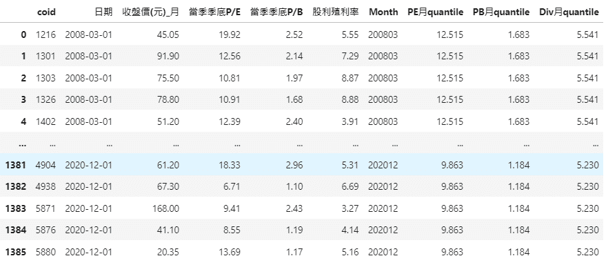
.reset_index(drop =True)After the selection, you can clearly see that our data has reduced from 2,419 to 1,386. Then we will present it to you in two sorted ways, one is by coid and the other one is by date.
(The codes and parameter explanation can mainly refer to the fourth step in [Application (1)]. Except for the time period and grouping, the remaining parameters and logical concepts are similar to this strategy.)
The strategy will change the portfolio every quarter. Since we can directly find the company’s quarterly return through the TWN/APRCD2 database in TEJ, we compare the quarterly return of each quarter of the portfolio and the quarterly return of 0050. The code is as follows:
*This backtest ignores all transaction costs.
import datetime
return_=pd.DataFrame()
dates = df_filter['日期'].astype(str).apply(lambda x: x.split(' ')[0]).unique()

for date in dates:

    # 設定日期
    year = int(date.split('-')[0])
    month = int(date.split('-')[1])
    day = 1
    date1 = str(year)+'-'+str(month)+'-'+str(day)
    ret = [date1]
    pf = df_filter[df_filter['日期']==date].reset_index(drop=True)
    print(date1)

    ## 將買進日期設在當月1日,由於報酬率的關係我們要找的時間為一季之後的報酬率當作是在原先時間購買持有的報酬率##
    buy_date = datetime.datetime(year,month,day) + datetime.timedelta(90)
    sell_date = buy_date + datetime.timedelta(90)
    pf_H = pf['coid'].to_list()
    print('getting data')
    data = tejapi.get('TWN/APRCD2',coid  = pf_H, paginate = True, mdate={'gte':buy_date,'lte':sell_date},chinese_column_name=True)
    q1_ret = data.groupby(by = '證券代碼').last()['季報酬率 %'].values

    # 計算報酬率 #
    print('calculating return')
    w = 1/len(pf_H) # 等權重
    q1_wret = (w*q1_ret).tolist() # 加權平均報酬
    ret.append(round(sum(q1_wret),2))

    ## 撈取台灣 50指數的年報酬率,日期設定為 buy_date(含)至 sell_date(含) ##
    tw0050 = tejapi.get('TWN/APRCD2',coid ='TRI50' ,paginate = True,mdate={'gte':buy_date,'lte':sell_date},chinese_column_name=True)
    bm_return = tw0050.groupby(by = '證券代碼').last()['季報酬率 %'].values
    if bm_return.size!=0:
        ret.append(round(bm_return.tolist()[0],2))
    else:
        ret.append(None)
    rets = np.reshape(np.array(ret),(1,3)).tolist()
    retss = pd.DataFrame(data=rets,columns=['Date','port_return','twn50_return'])
    return_ = return_.append(retss).reset_index(drop=True)
    print(return_)
Then we can watch our return table.
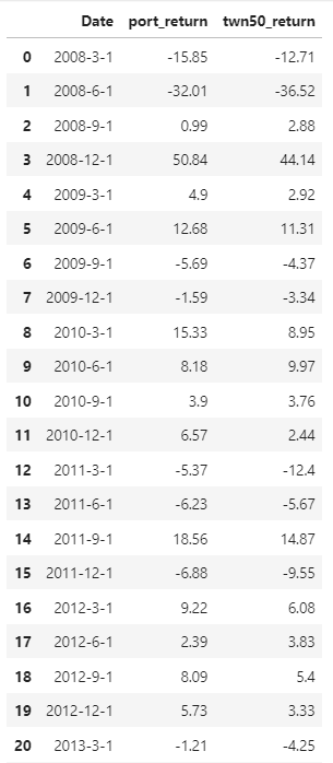
We will simply present the quarterly return and the cumulative return by the graphs to everyone.
##Quarterly return and cumulative return
cum_ret = ((return_[['port_return', 'twn50_return']].astype(float)*0.01)+1).cumprod()
cum_ret['Date'] = return_['Date']
cum_ret = cum_ret[:len(cum_ret)-1]
cum_ret = cum_ret[['Date','port_return','twn50_return']]
quarter_ret = return_[['port_return', 'twn50_return']].astype(float)
quarter_ret['Date'] = return_['Date']
quarter_ret = quarter_ret[:len(quarter_ret)-1]
quarter_ret = quarter_ret[['Date','port_return','twn50_return']]plt.style.use('seaborn')
plt.figure(figsize=(10,5))
plt.xticks(rotation = 90)
plt.title('master invest strategy - quarter return',fontsize = 20)
date = quarter_ret['Date']
plt.plot(date,quarter_ret.port_return,color ='red',label='port_return')
plt.plot(date,quarter_ret.twn50_return,color = 'black',label='twn50_return')
plt.legend(fontsize = 15)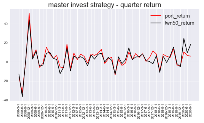
plt.style.use('seaborn')
plt.figure(figsize=(10,5))
plt.xticks(rotation = 90)
plt.title('master invest strategy - cumulative return',fontsize = 20)
date = cum_ret['Date']
plt.plot(date,cum_ret.port_return,color ='red',label='port_return')
plt.plot(date,cum_ret.twn50_return,color = 'black',label='twn50_return')
plt.legend(fontsize = 15)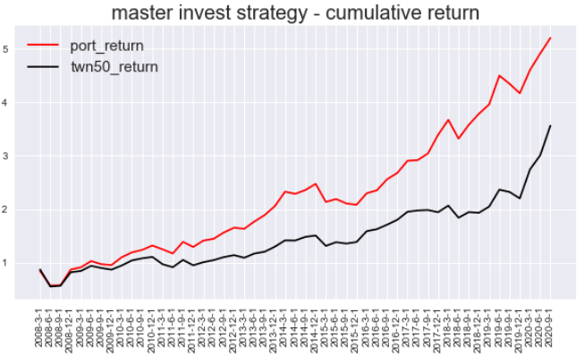
The performance of the master’s strategy is very outstanding!
Ratio = pd.DataFrame()
for col in cum_ret.columns[1:]:

    ##CAGR
    cagr = (cum_ret[col].values[-1]) ** (4/len(cum_ret)) -1

    ##STD
    std = return_[col][:len(return_)-1].astype(float).std()

    ##Sharpe Ratio(假設無風險利率為1%)
    sharpe_ratio = (cagr-0.01)/(std*0.01)

    ##MDD
    roll_max = cum_ret[col].cummax()
    monthly_dd =cum_ret[col]/roll_max - 1.0
    max_dd = monthly_dd.cummin()

    ##Table
    ratio = np.reshape(np.round(np.array([100*cagr, std, sharpe_ratio, 100*max_dd.values[-1]]),2),(1,4))
    Ratio = Ratio.append(pd.DataFrame(index=[col],
      columns=['年化報酬率(%)', '年化標準差(%)', '夏普比率', '期間最大回撤(%)'],
      data = ratio))
Ratio.T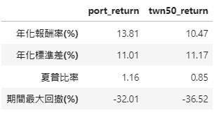
pf = df_filter[df_filter['日期']== '2020-12-01'].reset_index(drop=True)
stk_info['stk_num'] = stk_info['成份股'].apply(lambda x: str(x).split(' ')[0])
stk_info['stk_cname'] = stk_info['成份股'].apply(lambda x: str(x).split(' ')[1])
stk_info['成份股'][stk_info['stk_num'].isin(pf['coid'].tolist())].to_list()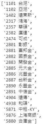
We have implemented several master strategies through python. In addition to data collation, we also backtested them and presented the results through tables and visualizations. Hope everyone can be satisfied with our articles.
To make successful backtesting, we still need to pay attention to things such as the data quality, the length of data, whether there are bugs in your program, whether too many transaction costs are ignored, etc. As long as there is a mistake in these problems, it will cause the distortion of the backtesting and lose money!! As a result, you have to pay attention to our backtesting result again️️️️️️️️️️️ every time.
Finally, if you like this topic, please click below, giving us more support and encouragement. Then, we will still work on financial data analysis and applications in the following articles, please look forward to them Besides, if you have any questions or suggestions, please leave a message or email us, we will try our best to reply to you.
Question:
Where could I get the data with a stable, high quality, and the time length is sufficient? TEJ API is your best choice!!
