
Table of Contents
Aroon Indicator, developed by Tushar Chande in 1995, is typically for measuring market tendency. It consists of two lines - Aroon Up and Aroon Down.
The Aroon Up indicator measures the strength and time since the highest price within a given period (usually 25 periods). In contrast, the Aroon Down indicator measures the strength and time since the lowest price within the same period. These indicators are expressed as percentages and range from 0% to 100%.
The crossover of the Aroon Up and Aroon Down lines can be used to signal potential changes in trend direction. For example, when Aroon Up crosses above Aroon Down, it might be seen as a bullish signal, indicating a potential shift towards an upward trend. Conversely, when Aroon Down crosses above Aroon Up, it could be interpreted as a bearish signal, suggesting a potential shift towards a downward trend.
When Aroon Up is greater than 80 and Aroon Down is lesser than 45, which represents a bullish trend. We consider it a buying signal and will acquire one unit at tomorrow’s opening price.
When Aroon Up is lesser than 45, Aroon Down is greater than 55, and the gap of two indicators is greater than 15, we regard it as a selling signal and sell the holding position at tomorrow’s opening price.
When Aroon Up is greater than 55, Aroon Down is lesser 45, the gap between the two indicators is greater than 15, our invested amount isn’t greater than 20% principal, and we still have plentiful cash. We will acquire one more unit at tomorrow’s opening price.
MacOS and Jupyter Notebook is used as editor
The back testing time period is between 2018/01/01 to 2020/12/31, and we take Hon Hai Precision Industry(2317), Compal Electronics(2324), Yageo Corporation(2327), TSMC(2330), Synnex(2347), Acer(2353), FTC(2354), ASUS(2357)、Realtek(2379), Quanta(2382), and Advantech(2395) to construct the portfolio and compare the performance of portfolio with the benchmark– Total. Return Index(IR0001), .
import os
import pandas as pd
import numpy as np
import tejapios.environ['TEJAPI_KEY'] = 'Your key'
os.environ['mdate'] = '20180101 20201231'
os.environ['ticker'] = 'IR0001 2317 2324 2327 2330 2347 2353 2354 2357 2379 2382 2395'!zipline ingest -b tquantfrom zipline.api import set_slippage, set_commission, set_benchmark, attach_pipeline, order, order_target, symbol, pipeline_output, record
from zipline.finance import commission, slippage
from zipline.data import bundles
from zipline import run_algorithm
from zipline.pipeline import Pipeline, CustomFactor
from zipline.pipeline.filters import StaticAssets, StaticSids
from zipline.pipeline.factors import BollingerBands, Aroon
from zipline.pipeline.data import EquityPricing
from zipline.pipeline.mixins import LatestMixin
from zipline.master import run_pipelineFirst, We load the bundle which we just ingest above, and set return index(coid : IR0001) as benchmark.
bundle = bundles.load('tquant')
ir0001_asset = bundle.asset_finder.lookup_symbol('IR0001',as_of_date = None)Pipeline() enables users to quickly process multiple assets’ trading-related data. In today’s article, we use it to process:
The calculation of Aroon-up, Aroon-down (built-in factor:Aroon)
def make_pipeline():
curr_price = EquityPricing.close.latest

alroon = Aroon(inputs = [EquityPricing.low, EquityPricing.high], window_length=25, mask = curr_price < 5000)
up, down = alroon.up, alroon.down return Pipeline(
columns = {
'up': up,
'down': down,
'curr_price': curr_price, },
screen = ~StaticAssets([ir0001_asset])
)inintialize enables users to set up the trading environment at the beginning of the back test period. In this article, we set up:
def initialize(context):
set_slippage(slippage.VolumeShareSlippage())
set_commission(commission.PerShare(cost=0.00285))
set_benchmark(symbol('IR0001'))
attach_pipeline(make_pipeline(), 'mystrategy')handle_data is used to process data and make orders daily.
Default trading signals buy and sell are False
buy: When today’s indicators matches the buy-in condition, generates buying signal and toggles the boolean value to True。sell: When today’s indicators matches the sell-out condition, generates selling signal and toggles the boolean value to True。def handle_data(context, data):
out_dir = pipeline_output('mystrategy')
for i in out_dir.index:
sym = i.symbol # 標的代碼
up = out_dir.loc[i, 'up']
down = out_dir.loc[i, 'down']
curr_price = out_dir.loc[i, 'curr_price'] cash_position = context.portfolio.cash
stock_position = context.portfolio.positions[i].amount buy, sell = False, False record(
**{
f'price_{sym}':curr_price,
f'up_{sym}':up,
f'down_{sym}':down,
f'buy_{sym}':buy,
f'sell_{sym}':sell
}
) if stock_position == 0:
if down < 45 and up > 80:
order(i, 1000)
context.last_signal_price = curr_price
buy = True
record(
**{
f'buy_{sym}':buy
}
) elif stock_position > 0:
if (up - down) > 15 and (down < 45) and (up > 55) and (cash_position >= curr_price * 1000):
order(i, 1000)
context.last_signal_price = curr_price
buy = True
record(
#globals()[f'buy_{sym}'] = buy
**{
f'buy_{sym}':buy
}
) elif (down - up > 15) and (down > 55) and (up < 45):
order_target(i, 0)
context.last_signal_price = 0
sell = True
record(
**{
f'sell_{sym}':sell
}
)
else:
pass
else:
passanalyzefunction is mostly used to visualize the result of backtesting. Since today’s practice will use pyfolio to achieve visualization, we just leave it empty.
def analyze(context, perf):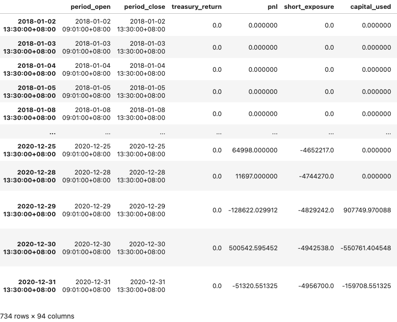
passWe expliot run_algorithm() to execute our strategy. The backtesting time period is set between 2018-01-01 to 2020–12–31. The data bundle we use is tquant. We assume the initial capital base is 1,000,000. The output of run_algorithm(), which is results, contains information on daily performance and trading receipts.
results = run_algorithm(
start = pd.Timestamp('2018-01-01', tz='UTC'),
end = pd.Timestamp('2020-12-31', tz ='UTC'),
initialize=initialize,
bundle='tquant',
analyze=analyze,
capital_base=10e6,
handle_data = handle_data
)
results
Before process visualization, we need to seperate the data of results to three part:
from pyfolio.utils import extract_rets_pos_txn_from_zipline
returns, positions, transactions = extract_rets_pos_txn_from_zipline(results)# 時區標準化
returns.index = returns.index.tz_localize(None).tz_localize('UTC')
positions.index = positions.index.tz_localize(None).tz_localize('UTC')
transactions.index = transactions.index.tz_localize(None).tz_localize('UTC')
benchmark_rets.index = benchmark_rets.index.tz_localize(None).tz_localize('UTC')
Lastly, pyfolio.tears.create_full_tear_sheet can generate multiple tables and charts to help you evaluate the portfolio’s performance.
pyfolio.tears.create_full_tear_sheet(returns=returns,
positions=positions,
transactions=transactions,
benchmark_rets=benchmark_rets)In this implementation, we have utilized TQuant Lab to implement the Aron indicator trading strategy. Compared to writing the code without using TQuant Lab, the program’s complexity has significantly decreased, and it offers more detailed parameter settings and evaluation metrics.
A friendly reminder that this strategy and the underlying assets are for reference purposes only and do not constitute any recommendations for commodities or investments. In the future, we will also introduce the use of the TEJ database to construct various indicators and backtest their performance. Therefore, we welcome readers interested in various trading backtesting to choose TEJ E-Shop’s relevant solutions and use high-quality databases to create their own trading strategies.
