
Table of Contents
Ichimoku Kinko Hyo (also known as Cloud Charts, いちもくきんこうひょう) was invented by Japanese journalist Goichi Hosoda, but it was not publicly disclosed at the time. Forty years later, between 1975 and 6 years after that, Goichi Hosoda, using the pseudonym Ichimoku Sanjin, published seven series of works under the name “Ichimoku Kinko Hyo,” explaining in detail this indicator and the philosophical thinking behind its trading system.
Unlike traditional concepts such as stock prices influenced by price-volume relationships, supply and demand for buying and selling, and fundamental aspects of companies, Ichimoku Kinko Hyo believes that time is an essential factor affecting price changes, especially under the influence of time, prices have cyclical changes. There is always a market concern that stocks will fall after rising for a long time and rise after falling for a long time. The overall market sentiment reflects a regularity of fluctuations in market behavior under the influence of time, which forms the basis of the “Time Theory” of Ichimoku Kinko Hyo.
In addition, Ichimoku Kinko Hyo is a philosophical, technical analysis indicator. Rather than being an indicator per se, the author believes it should be regarded as Goichi Hosoda’s analysis and reflection on the market and society. The thought behind it is worth exploring in depth. Due to space constraints, this article does not elaborate on this. The author believes that the theory of Ichimoku Kinko Hyo and market equilibrium has good insights into Ichimoku Kinko Hyo. Those interested can refer to it.
The time theory of Ichimoku Kinko Hyo is a method of analyzing time and market turning points. “9, 17, 26” are the basic numbers and can be used to examine whether the market will likely have a turning point during this period, which is a significant value.
tenkan_sen): The turning line (also known as the reversal line) is the average of the highest and lowest prices in the past nine days. If the turning line rises, it is judged that the upward momentum is strong, and if it falls, it is considered that the downward trend is strong. Because it is calculated based on a short period of nine days, it is used to analyze short-term trends.kijun_sen): The standard line is the average of the highest and lowest prices over the past 26 days. If the standard line rises, it is judged that the upward momentum is strong, and if it falls, it is considered that the downward trend is strong. Since it is calculated based on a period of 26 days, it is used to analyze medium-term trends.senkou_span_a/b): Leading Span A predicts the future trend for the next 26 days based on the average turning line and the standard line. Leading Span B is a line that predicts the trend for the next 26 days based on the average of the highest and lowest prices of the past 52 days. Since both show the average trend for the next 26 days, they help analyze future price changes. After shading between Leading Span A and Leading Span B, the “cloud region or cloud band” is called the part with A < B, green, and the part with A > B, red.chikou_span): The lagging span is the stock price 26 days ago. If it is above the price line, it indicates a strong upward trend in the market; if it is below the price line, it indicates a solid downward trend.Ichimoku Kinko Hyo also has a method called “Three-Line Confirmation” and “Three-Line Reversal” for interpreting. “Three-line confirmation” represents a buy signal, and “Three-Line Reversal” represents a sell signal. Usually, if the three-line confirmation is met outside the stock’s price range, there will be a stronger upward trend, and vice versa. This article will fine-tune the buy signal based on the three-line confirmation.
Conditions for Three-Line Confirmation:
Conditions for Three-Line Reversal:
This article uses MacOS and Jupyter Notebook as the editor.
get_universe Function to Obtain Stock PoolThis strategy first fetches all stock codes of common stocks, including both listed and over-the-counter (OTC) markets, for one year, from April 1, 2018, to March 31, 2019.
import os
import tejapi
import pandas as pd
import numpy as np

os.environ['TEJAPI_KEY'] = "your key"
os.environ['TEJAPI_BASE'] = "https://api.tej.com.tw"
start = '2018-04-01'
end = '2019-03-31'
from zipline.sources.TEJ_Api_Data import get_universe
pool = get_universe(start, end, mkt = ['TWSE', 'OTC'], stktp_e=['Common Stock-Foreign', 'Common Stock'])
len(pool)The Ichimoku Kinko Hyo strategy selects MSCI component stocks from the above stock codes using the TEJToolAPI.
average_vol = df.groupby('股票代碼')['成交量_千股'].mean().reset_index()
average_vol = average_vol.rename(columns={'成交量_千股': '平均成交量'})
high_price_stocks = df.groupby('股票代碼')['最低價'].min().reset_index()
high_price_stocks = high_price_stocks[high_price_stocks['最低價'] >= 50]
merge_data = pd.merge(average_vol, high_price_stocks, on='股票代碼', how='inner')
top_100_vol = merge_data.sort_values(by='平均成交量', ascending=False).head(100)
top_100_vol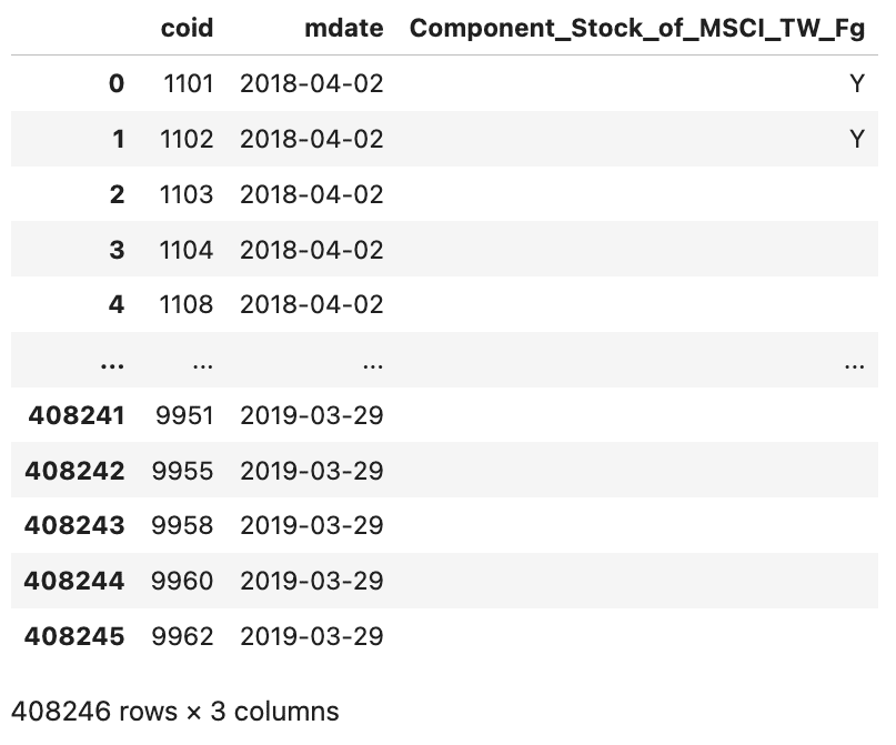
To avoid lookahead bias, this strategy’s five-year backtesting period is from April 1, 2019, to April 1, 2024. It includes the aforementioned 91 constituent stocks, along with the Taiwan Weighted Index (IR0001), as a benchmark for market comparison.
Below is the list of the 91 constituent stocks and the Taiwan Weighted Index:
!zipline ingest -b tquant
!zipline bundle-info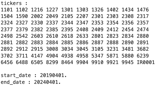
CustomFactor allows users to design custom factors as needed. In this case, we will use it to handle:
Average True Range (ATR): Used to calculate trailing stop levels. Pipeline allows users to process quantitative indicators and price-volume data for multiple assets quickly. In this case, we will use it to handle:
Conversion Line (tenkan_sen) Base Line (kijun_sen) Leading Span A / B (senkou_span_a/b) Cloud area or cloud band (cloud_red) Lagging Span (chikou_span)
from zipline.pipeline import Pipeline
from zipline.TQresearch.tej_pipeline import run_pipeline
def make_pipeline():

    Ich = IchimokuKinkoHyo(
        inputs = [TWEquityPricing.high, TWEquityPricing.low, TWEquityPricing.close],
        window_length = 52,
    )
    atr = AverageTrueRange(inputs = [TWEquityPricing.high, TWEquityPricing.low, TWEquityPricing.close],
        window_length = 52,
    )

    return Pipeline(
        columns = {
            'curr_price': TWEquityPricing.close.latest,
            "tenkan_sen": Ich.tenkan_sen,
            "kijun_sen": Ich.kijun_sen,
            "senkou_span_a": Ich.senkou_span_a,
            "senkou_span_b": Ich.senkou_span_b,
            'cloud_red': Ich.senkou_span_a < Ich.senkou_span_b,
            "chikou_span": Ich.chikou_span,
            'stop_loss': atr.ATR,
    },
        # screen = ~StaticAssets([benchmark_asset])
        screen = ~StaticAssets([benchmark_asset]) & (Ich.senkou_span_a > 0) & (Ich.senkou_span_b > 0)
    )
my_pipeline = run_pipeline(make_pipeline(), start_dt, end_dt)
my_pipeline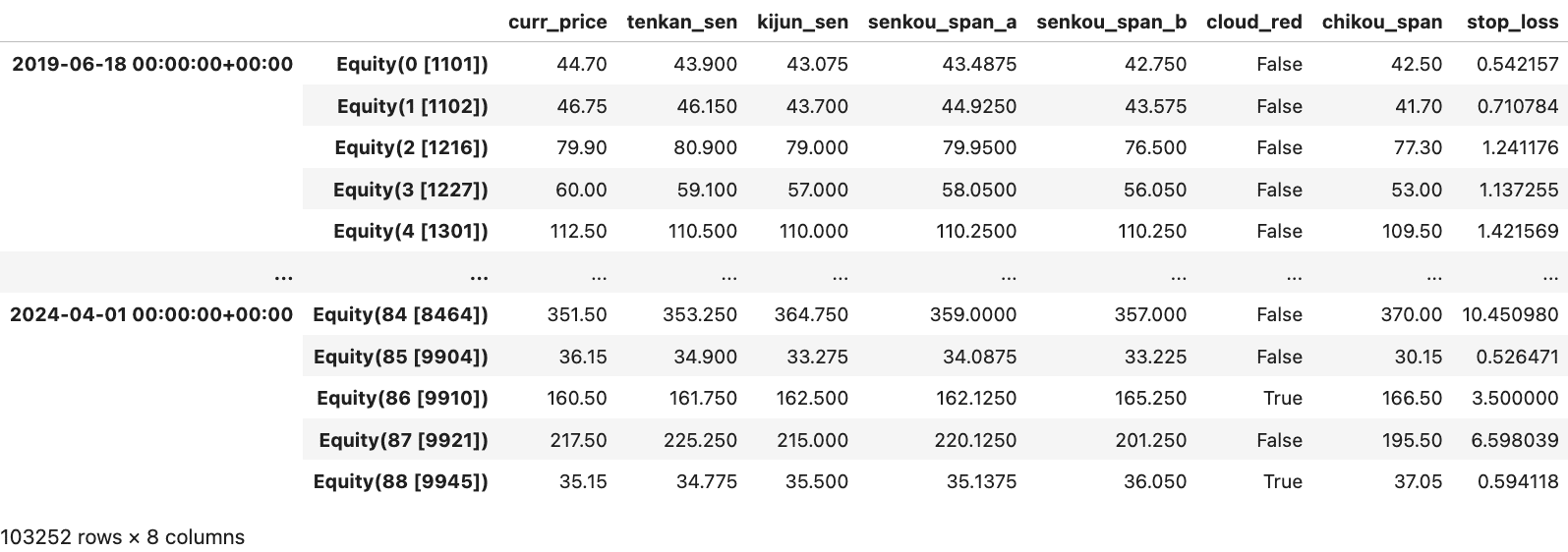
The initialize() function defines the daily trading environment before trading begins. In this example, we set:
context.stop_loss variable to record stop-loss points during backtestingcontext.holding variable to record whether a position in a particular stock is heldcontext.trailing_stop variable to record whether the trailing stop is being appliedcontext.last_buy_price variable to record the last purchase pricecontext.trailing_count variable to record the number of trailing stop instancescontext.buy_count variable to limit the maximum number of trades per stockfrom zipline.finance import slippage, commission
from zipline.api import *
def initialize(context):
set_slippage(slippage.VolumeShareSlippage())
set_commission(commission.Custom_TW_Commission(min_trade_cost = 20, discount = 1.0, tax = 0.003))
attach_pipeline(make_pipeline(), 'mystrats')
set_benchmark(symbol('IR0001'))
context.stop_loss = {}
context.trailing_stop = {}
context.last_buy_price = {}
context.trailing_count = {}
context.holding = {}
context.buy_count = {}The handle_data() function is important for constructing the Ichimoku Kinko Hyo strategy. It is called every day after the start of backtesting, and its main tasks include setting trading strategies, placing orders, and recording trading information.
Note: To avoid the possibility of erroneous entry signals by the Ichimoku Kinko Hyo during periods of price consolidation, this article uses an additional *1.01 condition on tenkan_sen > kijun_sen. This is done in the hope of entering the market only when the upward trend is sufficiently explicit, thereby achieving a certain degree of avoidance of consolidation periods.
For detailed trading rules regarding this strategy, please refer to Ichimoku Kinko Hyo.ipynb
        # 三役好轉 (tenkan_sen > kijun_sen*1.015 : avoid the Darvas Box Theory)
        if (curr_price > senkou_span_b) and (cloud_red == True) and (tenkan_sen > kijun_sen*1.01) and (context.buy_count[f'{i}'] <= 5):
            order_percent(i, 0.01)
            buy = True
            context.stop_loss[f'{i}'] = curr_price - (1.25 * stop_loss)
            context.last_buy_price[f'{i}'] = curr_price
            record(
                **{
                    f'buy_{sym}':buy
                }
            )
            context.holding[f'{i}'] = True
            context.buy_count[f'{i}'] += 1

        # reset stop loss point
        if (curr_price >= (1.3**context.trailing_count[f'{i}'])*context.last_buy_price[f'{i}']) and (context.holding[f'{i}'] == True) and (context.trailing_stop[f'{i}'] == False):
            context.stop_loss[f'{i}'] = 1.3*context.stop_loss[f'{i}']
            context.trailing_stop[f'{i}'] = True
            context.trailing_count[f'{i}'] += 1
        elif (curr_price >= (1.3**context.trailing_count[f'{i}'])*context.last_buy_price[f'{i}']) and (context.holding[f'{i}'] == True) and (context.trailing_stop[f'{i}'] == True):
            context.stop_loss[f'{i}'] = 1.3*context.stop_loss[f'{i}']
            context.trailing_count[f'{i}'] += 1

        if (curr_price <= context.stop_loss[f'{i}']) and (context.holding[f'{i}'] == True):
            order_target(i, 0)
            sell = True
            context.stop_loss[f'{i}'] = None
            context.trailing_stop[f'{i}'] = None
            context.trailing_count[f'{i}'] = None
            record(
                **{
                    f'sell_{sym}':sell
                }
            )
            context.holding[f'{i}'] = None
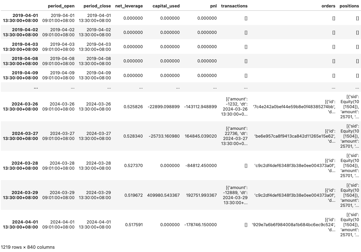
context.buy_count[f'{i}'] = NoneUse the run_algorithm() function to execute the Ichimoku Kinko Hyo strategy as defined above. Set the trading period from start_dt (2019-04-01) to end_dt (2024-04-01), using the dataset tquant, with an initial capital of 20 million dollars. The output results represent the daily performance and trade details.
import matplotlib.pyplot as plt
from zipline import run_algorithm

results = run_algorithm(
    start = start_dt,
    end = end_dt,
    initialize = initialize,
    bundle = 'tquant',
    analyze = analyze,
    capital_base = 2e7,
    handle_data = handle_data
)

results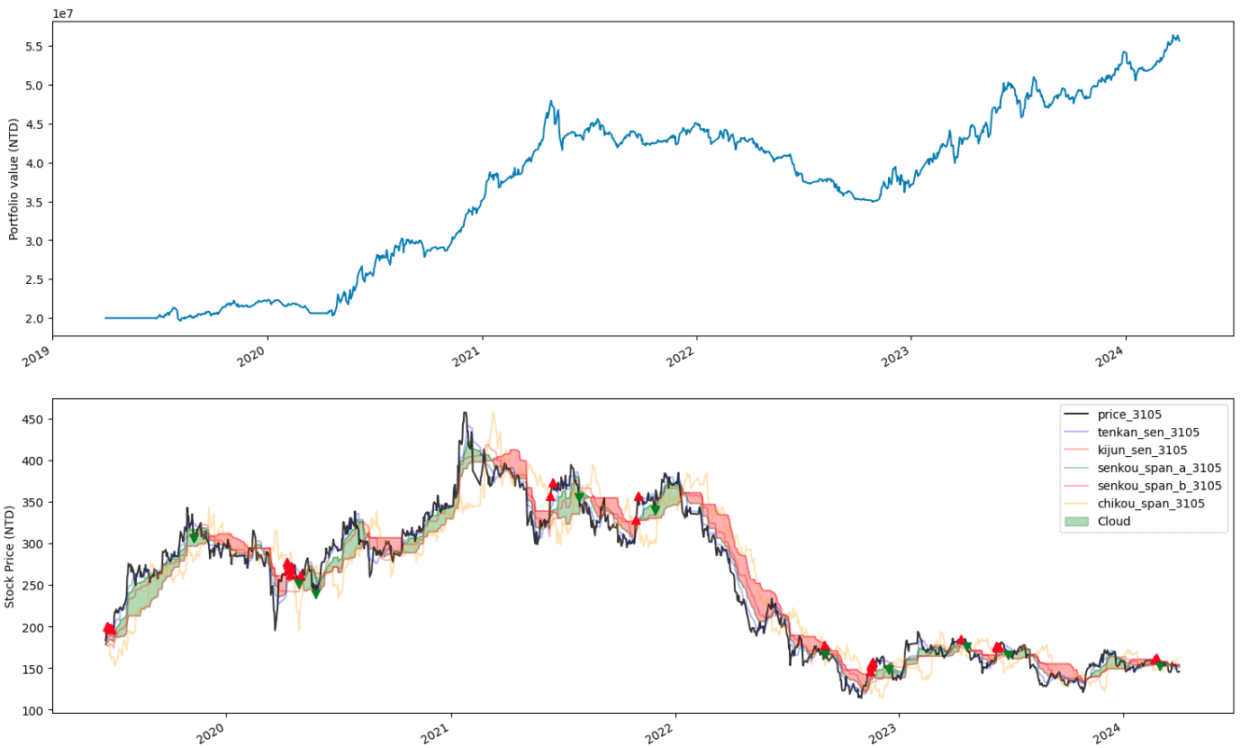
import pyfolio as pf
returns, positions, transactions = pf.utils.extract_rets_pos_txn_from_zipline(results)
benchmark_rets = results['benchmark_return']
pf.tears.create_full_tear_sheet(returns=returns,
                                positions=positions,
                                transactions=transactions,
                                benchmark_rets=benchmark_rets
                                )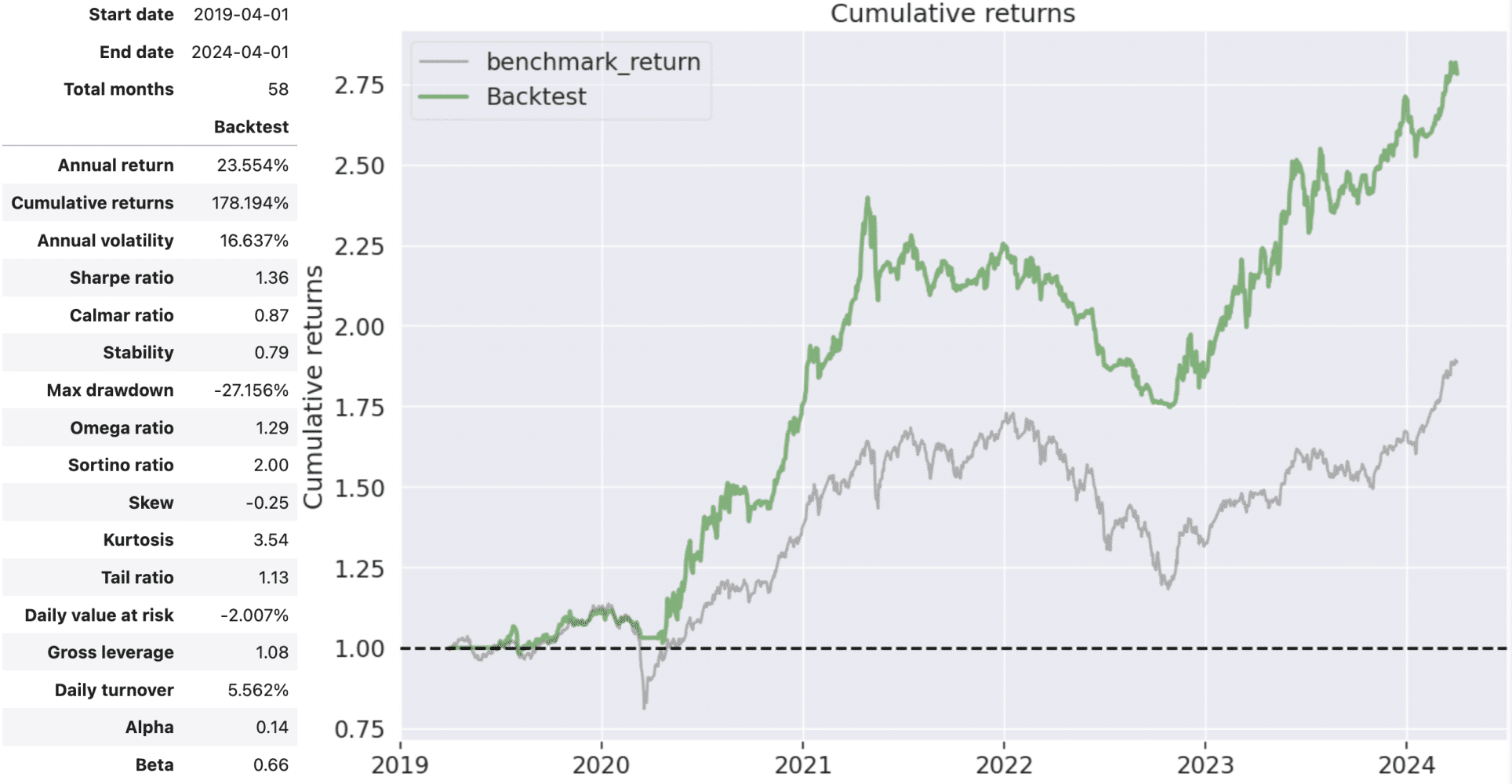
We can observe that the Ichimoku Kinko Hyo strategy has provided excellent performance over the 58 months, with an annualized return of 23.554% and a cumulative return of 178.194%. The profit performance is quite impressive. The Sharpe ratio 1.38 indicates a relatively high return compared to the risk. Additionally, the β value of 0.66 suggests that the strategy’s volatility is relatively insensitive to overall market volatility, reflecting the core concept of the Ichimoku Kinko Hyo system in detaching from the market.
Regarding maximum drawdown, we can see a significant downturn during the systemic risk increase due to the epidemic between the 22nd and 23rd years. Stable growth trends have characterized other periods. Utilizing the entry signals provided by the Ichimoku Kinko Hyo, along with a strategy incorporating ATR trailing stops, is a robust approach for achieving consistent returns surpassing the market over the long term.

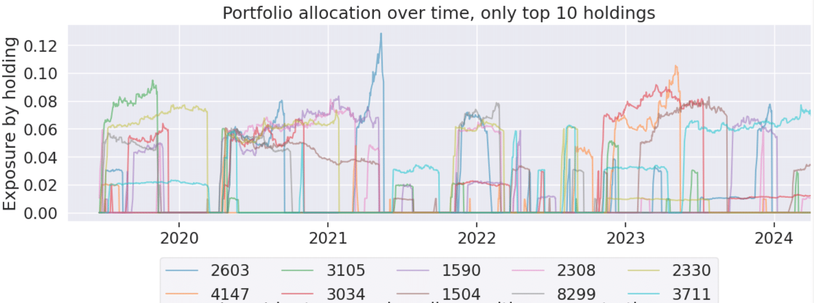
It can be seen that the holding period for each stock is quite consistent, with little bias towards any particular stock.
graph(2330, True)Since this strategy involves backtesting on a selection of stocks rather than individual stock backtesting, it’s impossible to quickly ascertain the actual entry and exit points for each stock within the Ichimoku Kinko Hyo system. Therefore, I have additionally written a function to facilitate the examination of individual stock trading situations. For more details, please refer to the source code on GitHub.

A notable point is that the entry method based on Ichimoku Kinko Hyo’s three signals does not include exit criteria. In practical testing, exiting based on the reversal of the three signals would result in losing many profitable trends. Therefore, this strategy employs a trailing stop-loss method for exits. For instance, in the chart above, you can see that the strategy had a sell order triggered by a stop-loss signal on TSMC (2330) at the beginning of 2021, capturing a trend lasting over half a year. However, apart from trailing stop-loss, one could incorporate profit-taking mechanisms such as setting profit targets or other means of securing gains. Additionally, strategies involving both long and short positions could be explored.
This strategy uses the Ichimoku Kinko Hyo for backtesting simulations, leveraging its signals of three conversions for entry and complementing it with trailing stop-loss for profit-taking, yielding promising backtest results. Investors are welcome to consider this approach.
In the future, I will continue to introduce various indicators constructed using the TEJ database and backtest their performance. Therefore, readers interested in trading backtests are encouraged to explore TQuant Lab‘s related solutions, utilizing high-quality databases to build their trading strategies.
A friendly reminder: This strategy is for reference only and does not constitute any recommendation for commodities or investments.
[TQuant Lab] Solving Your Quantitative Finance Pain Points
Comprehensively providing all the tools needed for trading backtesting.