Table of Contents
The KD Indicator, also known as the Stochastic Oscillator, is a practical and widely used tool in technical analysis. It’s primarily used to determine the short-term strength of stock prices and potential reversal timing. The value of the KD indicator ranges from 0 to 100, with 50 generally serving as the dividing line. When the indicator is above 50, it indicates that the stock price is in a bullish phase; conversely, when the indicator is below 50, it is considered to be in a bearish phase. Additionally, when the KD indicator is below 20, stocks often show signs of being oversold, indicating a potential upward reversal at any time; on the other hand, when the KD indicator is above 80, stocks often exhibit signs of being overbought, suggesting a potential downward reversal at any time. Therefore, this tool is a valuable resource for constructing trading signals for buying and selling stocks, empowering traders with timely and informed decisions.
The calculation process of the KD indicator is as follows:
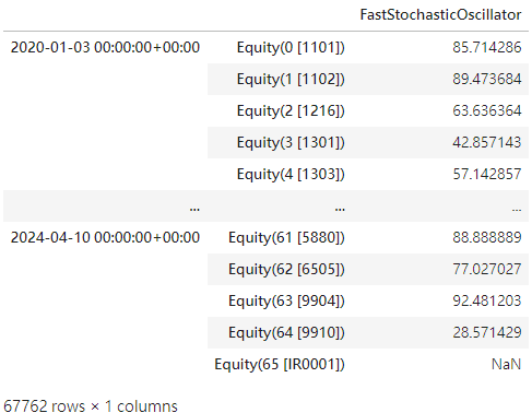
From the above formulas, RSV can be interpreted as the strength or weakness of today’s stock price relative to the prices over the past N days. K value, also known as the Fast Stochastic Oscillator, is heavily influenced by the strength or weakness of today’s stock price. On the other hand, the calculation principle of D value is akin to applying another level of smoothing. Hence, it reacts more slowly to current price changes.
Moreover, the value of N in the equations represents the moving window for calculating the indicator. This value can be adjusted according to different investment characteristics, offering a flexible and versatile approach. Setting a larger N value can stabilize the KD values and provide more precise reversal signals based on a more extended historical period, which is suitable for medium- to long-term investors. Conversely, a smaller N value will make the KD indicator more sensitive and suitable for short-term investors. This adaptability allows the KD Indicator to cater to a wide range of investment strategies, making it a valuable tool for all types of traders.
In this article, we employ the KD indicator to determine stock price reversal timing and utilize the following entry and exit rules to establish a trading strategy and conduct backtesting:
Additionally, since this strategy involves a longer backtesting period, the value of N is 36 days instead of the more common 14-day window length used in calculating the KD indicator.
This article is written using Windows 11 and Jupyter Lab as the editor.
import pandas as pd
import numpy as np
import os

tej_key = 'your key'
api_base = 'https://api.tej.com.tw'

os.environ['TEJAPI_KEY'] = tej_key
os.environ['TEJAPI_BASE'] = api_baseget_universe to select stocks from the Taiwan 50 Index from 2012-01-01 to 2019-12-31.!zipline ingest -b tquant.from zipline.sources.TEJ_Api_Data import get_universe
# get the stock list from Taiwan 50 index
StockList = get_universe('2012-01-01', '2019-12-31', idx_id = 'IX0002')
StockList.append('IR0001')
# set backtest period
start = '2020-01-01'
end = '2024-04-10'
os.environ['ticker'] = ' '.join(StockList)
os.environ['mdate'] = start + ' ' + end
!zipline ingest -b tquantFrom the pipeline and zipline function provided in TQuant Lab, we can:
pipeline.
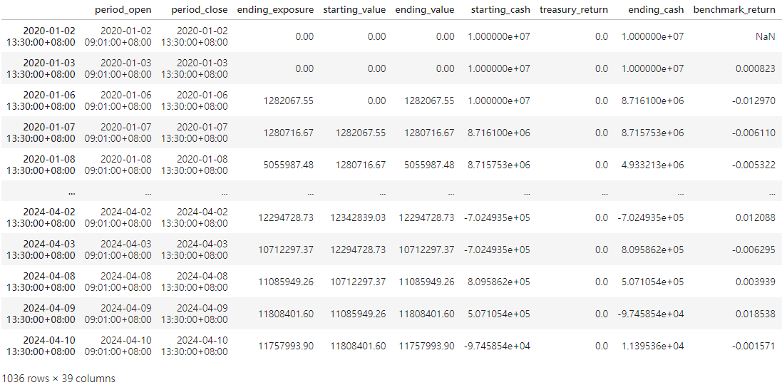
We use run_algorithm() function to execute the configured KD Indicator Strategy with the trading period from 2020-01-01 to 2024-04-10 and with the initial capital of 10,000,000 NTD. The output, or results, will represent the daily performance and detailed transaction records.
from zipline import run_algorithm

start_date = pd.Timestamp('2020-01-01',tz='utc')
end_date = pd.Timestamp('2024-04-10',tz='utc')

results = run_algorithm(start = start_date,
                        end = end_date,
                        initialize = initialize,
                        capital_base = 1e7,
                        handle_data = handle_data,
                        data_frequency = 'daily',
                        bundle = 'tquant'
                        )
results
import pyfolio as pf

returns, positions, transactions = pf.utils.extract_rets_pos_txn_from_zipline(results)
benchmark_rets = results.benchmark_return

# Creating a Full Tear Sheet
pf.create_full_tear_sheet(bt_returns, positions = positions, transactions = transactions,
                          benchmark_rets = benchmark_rets)
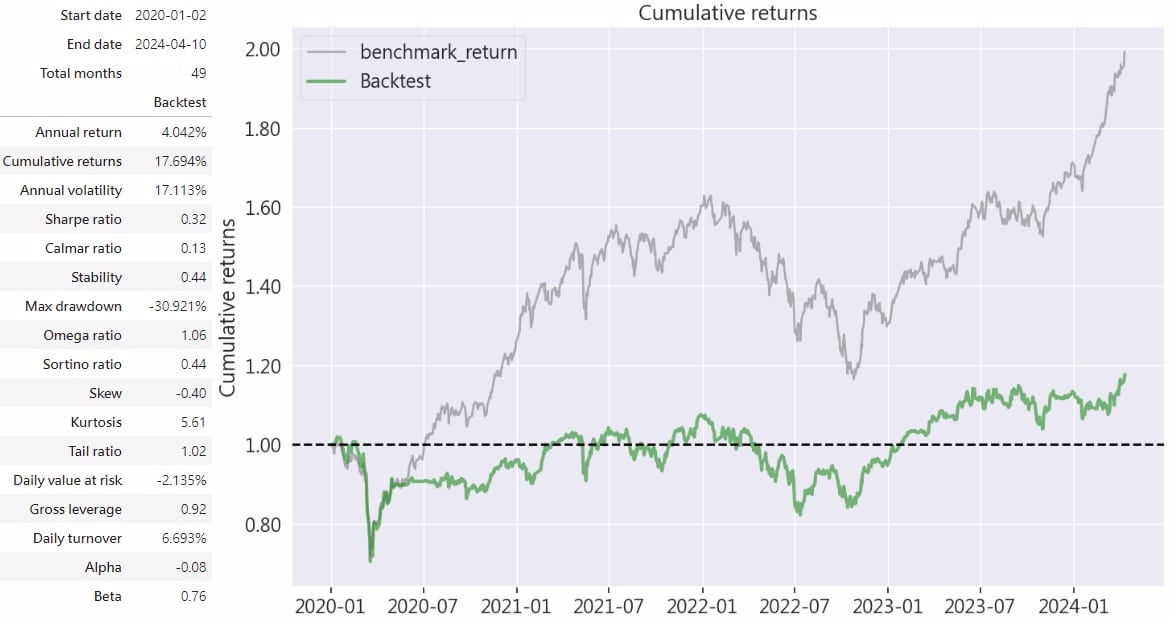
Through the above chart, it can be observed that the market has doubled its returns over the past four years. In contrast, the KD Indicator Strategy only achieved a cumulative return of approximately 17.7%. The annualized return rate and annualized volatility were 4% and 17.1% respectively. This has resulted in a performance gap between the KD Indicator Strategy and the market during the backtesting period. The author believes there are three main reasons for this:
Regarding the above three points, we can improve the KD Indicator Strategy by combining it with other indicators, such as factors that assist in identifying indicator divergences ( for application of indicator divergences, please refer to TQuant Lab RSI Moving Average Strategy – Identifying Reversals in Oversold Conditions ), or by integrating indicators like MACD. We will leave this for further exploration in the future.
This strategy was inspired by the KD Indicator, utilizing TQuant Lab to incorporate multiple stocks and the built-in factor library of Pipeline to accelerate calculating the K value required for the KD Indicator Strategy. Subsequently, the backtesting of the KD Indicator Strategy was conducted. Although the backtest results were not entirely satisfactory, we observed three drawbacks of the KD Indicator Strategy: indicator lag, missed timing of buying and selling points, and the generation of false trading signals. Investors should also be mindful of these situations when using the KD indicator. Otherwise, combining it with other indicators to assist in entry and exit decisions is preferable.
Please note that the strategy and target discussed in this article are for reference only and do not constitute any recommendation for specific commodities or investments. In the future, we will also introduce using the TEJ database to construct various indicators and backtest their performance. Therefore, we welcome readers interested in various trading strategies to consider purchasing relevant solutions from TQuant Lab. With our high-quality databases, you can construct a trading strategy that suits your needs.
[TQuant Lab] Solving Your Quantitative Finance Pain Points
Comprehensively providing all the tools needed for trading backtesting.