Table of Contents
In recent years, momentum trading has become a frequent topic of discussion in stock market strategies. In the stock market, we often hear discussions about the price-volume relationship, where price is considered a leading indicator of volume, among other concepts. This article aims to explore the backtesting effects of increasing trading volume as an entry strategy. Unlike some additional technical indicators that have predefined criteria, this method is designed to be more flexible, allowing readers to make their own adjustments in programming. Detailed parameter settings for customization will be mentioned in the later part of the code. This article employs the following strategy for backtesting:
This article is written using Windows 11 and Jupyter Notebook as the editor.
import pandas as pd
import numpy as np
import tejapi
import os
import pyfolio as pf
from zipline.api import set_slippage, set_commission, set_benchmark, attach_pipeline, order, order_target, symbol, pipeline_output
from zipline.finance import commission, slippage
from zipline.data import bundles
from zipline import run_algorithm
from zipline.pipeline import Pipeline
from zipline.pipeline.filters import StaticAssets
from zipline.pipeline.factors import SimpleMovingAverage
from zipline.pipeline.data import EquityPricingSet the following environment variables:
Then use the command !zipline ingest -b tquant to fetch the data.
os.environ['TEJAPI_BASE'] = 'https://api.tej.com.tw'
os.environ['TEJAPI_KEY'] = 'yourkey'
os.environ['mdate'] = '20120702 20220702'
os.environ['ticker'] = 'IR0001 2330 3443 2337'

!zipline ingest -b tquantThe Pipeline() function allows users to simultaneously process various quantitative indicators and price-volume data related to different assets. In this case, we use it to handle:
Additionally, we use screen and StaticAssets to filter out the broad market data (IR0001) during the daily calculation of the above indicators. This allows us to skip the calculation of the market index when computing the four-day simple moving average of trading volume, a five-day simple moving average of trading volume, and the daily trading volume for each stock.
bundle = bundles.load('tquant')
ir0001_asset = bundle.asset_finder.lookup_symbol('IR0001',as_of_date = None)

def make_pipeline():
    sma_vol_win_4 = SimpleMovingAverage(inputs=[EquityPricing.volume], window_length=4)
    sma_vol_win_5 = SimpleMovingAverage(inputs=[EquityPricing.volume], window_length=5)
    curr_vol = EquityPricing.volume.latest

    return Pipeline(
        columns = {
            'sma_4':sma_vol_win_4,
            'sma_5':sma_vol_win_5,
            'curr_vol':curr_vol
        },
        screen = ~StaticAssets([ir0001_asset])
)The initialize function is used to define the daily trading environment before trading begins. In this example, we set:
def initialize(context):
    set_slippage(slippage.VolumeShareSlippage())
    set_commission(commission.PerShare(cost=0.00285))
    set_benchmark(symbol('IR0001'))
attach_pipeline(make_pipeline(), 'mystrategy')The handle_data function is used to handle daily trading strategies or actions. In this function:
condition1: If the daily trading volume is greater than 2.5 times the four-day simple moving average and the cash position is greater than 0, generate a buy signal.condition2: If the daily trading volume is less than 0.75 times the five-day simple moving average, generate a sell signal.def handle_data(context, data):
out_dir = pipeline_output('mystrategy')
for i in out_dir.index:
sma_vol_4 = out_dir.loc[i, 'sma_4']
sma_vol_5 = out_dir.loc[i, 'sma_5']
curr_vol = out_dir.loc[i, 'curr_vol']
condition1 = (curr_vol > 2.5 * sma_vol_4) and (context.portfolio.cash > 0)
condition2 = (curr_vol < 0.75 * sma_vol_5)
if condition1:
order(i, 10)
elif condition2:
order_target(i, 0)
else:
passThe analyze function is typically used for generating performance charts. In this case, it will be used for plotting with pyfolio, so it can be skipped in this example.
def analyze(context, perf):
    pass
You can execute the trading strategy using the run_algorithm function with the settings you provided. Here’s a sample code snippet to run the strategy from July 2, 2012, to July 2, 2022, using the TQuant dataset with an initial capital of NTD 10,000. The results, including daily performance and trade details, will be stored in the results variable.
results = run_algorithm(
    start = pd.Timestamp('2012-07-02', tz='UTC'),
    end = pd.Timestamp('2022-07-02', tz ='UTC'),
    initialize=initialize,
    bundle='tquant',
    analyze=analyze,
    capital_base=1e4,
    handle_data = handle_data
)

results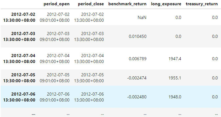
Then, we use pyfolio to visualize and analyze performance. At first, we can use extract_rets_pos_txn_from_zipline to separate above results data frame into 3 categories:
from pyfolio.utils import extract_rets_pos_txn_from_zipline
returns, positions, transactions = extract_rets_pos_txn_from_zipline(results)
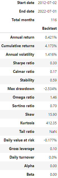
Use show_perf_stats() to generate portfolio performance table, this function enables us to quickly calculate the portfolio`s performance and risk. For detailed source code, please check out the GitHub hyperlink below.
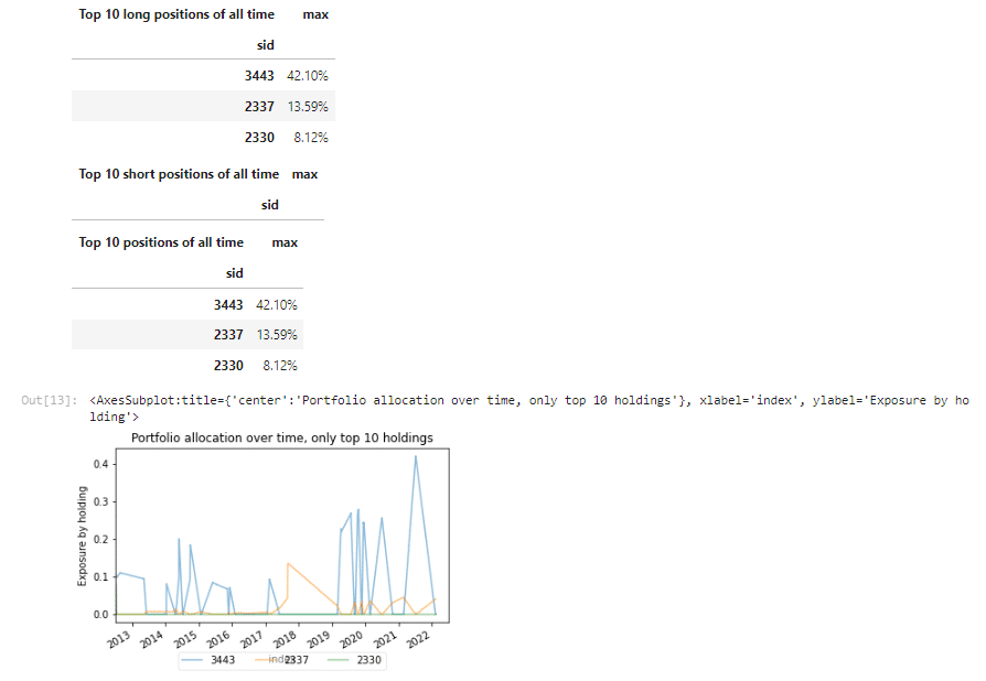
With show_and_plot_top_positions() and get_percent_alloc(), one can visualize the portfolio components easily. For detailed source code, please check out the GitHub hyperlink below.
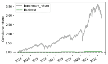
With plot_rolling_returns(), one can plot the cumulative returns for portfolio and benchmark. For detailed source code, please check out the GitHub hyperlink below.
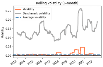
With plot_rolling_volatility(), one can plot the six-month rolling volatility for portfolio and benchmark. For detailed source code, please check out the GitHub hyperlink below.
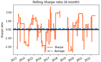
With plot_rolling_sharpe(), one can plot the six-month rolling Sharpe ratio for portfolio and benchmark. For detailed source code, please check out the GitHub hyperlink below.