
Table of Contents
The Price Deviation Ratio is a common technical indicator that compares the current stock price to the N-day moving average price, reflecting whether the current price is relatively high or low compared to its historical values. Generally, when the stock price consistently exceeds the moving average price, it’s called a ‘positive deviation.’ Conversely, it’s called’ negative deviation’ when it consistently falls below the moving average price.’ Therefore, when positive or negative deviation expands, it is interpreted as a sustained overbought or oversold condition in the market, serving as a basis for entry and exit decisions. However, using only the Price Deviation Ratio can generate too many trading signals. Hence, we include the highest and lowest prices over the past N days as a second filter. The actual strategy is as follows:
When the closing price is higher than the highest price over the past N days, and the Price Deviation Ratio is negative, enter a long position at the next day’s opening price.
When the closing price is lower than the lowest price over the past N days, and the Price Deviation Ratio is positive, exit the position and close the trade at the next day’s opening price.
This article uses MacOS and employs Jupyter as the editor.
import os
import pandas as pd
import numpy as np
import tejapi
import matplotlib.pyplot as pltThe back testing time period is between 2005/07/02 to 2023/07/02, and we take TSMC(2330) as an example.
os.environ['TEJAPI_BASE'] = 'https://api.tej.com.tw'
os.environ['TEJAPI_KEY'] = 'your_key'
os.environ['mdate'] = '20050702 20230702'
os.environ['ticker'] = '2330'
!zipline ingest -b tquantfrom zipline.api import (set_slippage,
set_commission,
set_benchmark,
attach_pipeline,
symbol,
pipeline_output,
record,
order,
order_target
)
from zipline.pipeline.filters import StaticSids
from zipline.finance import slippage, commission
from zipline import run_algorithm
from zipline.pipeline import CustomFactor, Pipeline
from zipline.pipeline.data import EquityPricing
from zipline.pipeline.factors import ExponentialWeightedMovingAveragePipeline() enables users to quickly process multiple assets’ trading-related data. In today’s article, we use it to process:
NdaysMaxHigh)NdaysMinLow)def make_pipeline():
ema = ExponentialWeightedMovingAverage(inputs = [EquityPricing.close],window_length = 7,decay_rate = 1/7)
high = NdaysMaxHigh(inputs = [EquityPricing.close], window_length = 8) # window_length 設定為 8,因為 factor 會包含當日價格。
low = NdaysMinLow(inputs = [EquityPricing.close], window_length = 8)
close = EquityPricing.close.latest
return Pipeline(
columns = {
'ema':ema,
'highesthigh':high,
'lowestlow':low,
'latest':close
}
)
class NdaysMaxHigh(CustomFactor):
def compute(self, today, assets, out, data):
out[:] = np.nanmax(data[:-2], axis=0)
class NdaysMinLow(CustomFactor):
def compute(self, today, assets, out, data):
out[:] = np.nanmin(data[:-2], axis=0)Initialize() enables users to set up the trading environment at the beginning of the back test period. In this article, we set up :
Pipline() function into back testing.def initialize(context):
set_slippage(slippage.VolumeShareSlippage())
set_commission(commission.PerShare(cost=0.00285))
set_benchmark(symbol('2330'))
attach_pipeline(make_pipeline(), 'mystrategy')handle_data() is used to process data and make orders daily.
def handle_data(context, data):

pipe = pipeline_output('mystrategy')

for i in pipe.index:
ema = pipe.loc[i, 'ema']
highesthigh = pipe.loc[i, 'highesthigh']
lowestlow = pipe.loc[i, 'lowestlow']
close = pipe.loc[i, 'latest']
bias = close - ema
residual_position = context.portfolio.positions[i].amount # 當日該資產的股數
condition1 = (close > highesthigh) and (bias > 0) and (residual_position > 0) # 賣出訊號
condition2 = (close < lowestlow) and (bias < 0) # 買入訊號

record( # 用以紀錄以下資訊至最終產出的 result 表格中
con1 = condition1,
con2 = condition2,
price = close,
ema = ema,
bias = bias,
highesthigh = highesthigh,
lowestlow = lowestlow
)

if condition1:
order_target(i, 0)
elif condition2:
order(i, 10)
else:
passHere, we apply matplotlib.pyplot for the trading signals and the portfolio value visualization.
def analyze(context, perf):
fig = plt.figure()
ax1 = fig.add_subplot(211)
perf.portfolio_value.plot(ax=ax1)
ax1.set_ylabel("Portfolio value (NTD)")
ax2 = fig.add_subplot(212)
ax2.set_ylabel("Price (NTD)")
perf.price.plot(ax=ax2)
ax2.plot( # 繪製買入訊號
perf.index[perf.con2],
perf.loc[perf.con2, 'price'],
'^',
markersize=5,
color='red'
)
ax2.plot( # 繪製賣出訊號
perf.index[perf.con1],
perf.loc[perf.con1, 'price'],
'v',
markersize=5,
color='green'
)
plt.legend(loc=0)
plt.gcf().set_size_inches(18,8)
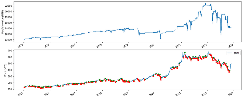
plt.show()We expliot run_algorithm() to execute our strategy. The backtesting time period is set between 2015–01–06 to 2022–11–25. The data bundle we use is tquant. We assume the initial capital base is 10,000. The output of run_algorithm(), which is results, contains information on daily performance and trading receipts.
results = run_algorithm(start = pd.Timestamp('20150106', tz='UTC'),
end = pd.Timestamp('20221125', tz='UTC'),
initialize=initialize,
bundle='tquant',
analyze=analyze,
capital_base=1e4,
handle_data = handle_data
)
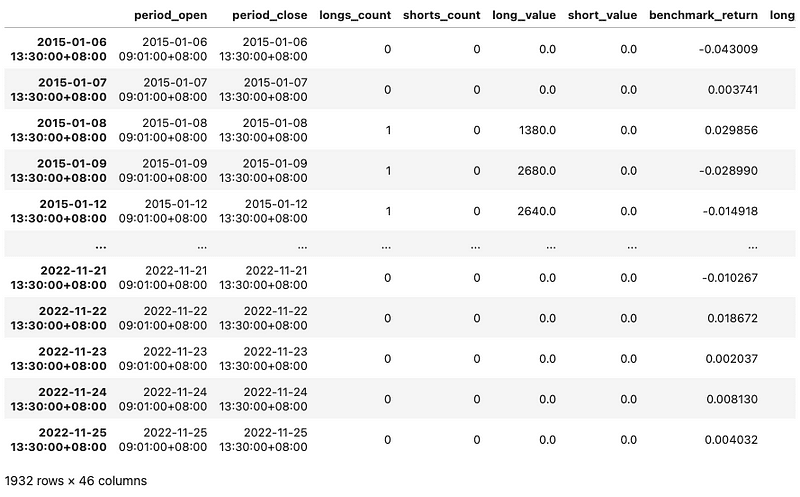
Then, we used Pyfolio module which came with TQuant Lab to analyze strategy`s performance and risk. First, we use extract_rets_pos_txn_from_zipline() to calculate returns, positions, and trading records.
import pyfolio as pf
returns, positions, transactions = pf.utils.extract_rets_pos_txn_from_zipline(results)Calculating daily portfolio return.
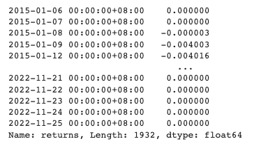
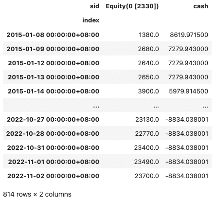
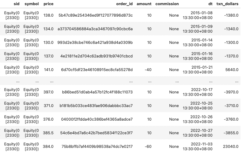
With show_perf_stats(), one can easily showcase the performance and risk analysis table.
import pyfolio as pf
pf.plotting.show_perf_stats(
returns,
benchmark_rets,
positions=positions,
transactions=transactions)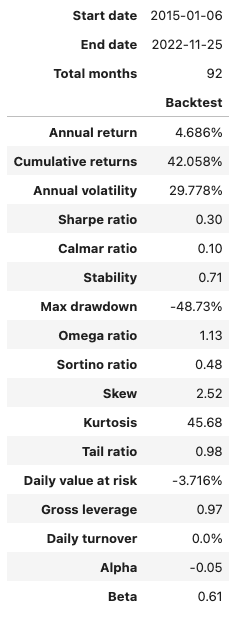
benchmark_rets = results['benchmark_return']
pf.plotting.plot_rolling_returns(returns, factor_returns=benchmark_rets)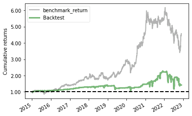
The strategy introduced in this session is one of the mean-reversion trading strategies. When the market is oversold (Bullish Divergence, BDI < 0), and the closing price is higher than the highest price over a certain period, it’s assumed that the stock price will gradually return to the moving average price, so a long position is entered. Conversely, when the stock price is overbought (Bearish Divergence, BDI > 0), and the closing price is lower than the lowest price over a certain period, it’s believed that the stock price has risen too much and has a downward trend. In this case, the long position is exited. However, it’s important to note that this strategy involves frequent trading, which transaction costs and taxes can erode. Therefore, it’s recommended to combine other technical indicators to optimize entry and exit points.
Finally, it’s worth mentioning again that the stocks discussed in this article are for illustrative purposes only and do not constitute recommendations for any financial products. If readers are interested in topics such as building strategies, performance backtesting, and empirical research, you are welcome to purchase solutions from TEJ E-Shop, which provides comprehensive databases to easily perform various tests and analyses.