Table of Contents
Look-ahead bias is the phenomenon that unconsciously uses unavailable or unrevealed data in analyzing or simulating historical events.
It exists in the processes of making decisions or evaluations which use information or data that was unknown at that time.
Look-ahead bias may cause distortion and misleadingness of the result because it violates the principle of using only information available during analysis. It could emerge in any field, such as finance, economy, and data analysis, and influence investment strategy, backtesting of the trading system, and performance grading.
Today’s practice will demonstrate a typical scenario of Look-ahead bias ━ using historical data, which contains the info of future variety in testing trading strategy. However, the info is unrevealed during the period of testing. This phenomenon may cause man-made overestimated performance and unrealistic expectations of the strategy’s profitability.
MacOS and Jupyter Notebook is used as editor
import pandas as pd
import re
import numpy as np
import tejapi
from functools import reduce
import matplotlib.pyplot as plt
from collections import defaultdict, OrderedDict
from tqdm import trange, tqdm
import plotly.express as px
import plotly.graph_objects as go
tejapi.ApiConfig.api_key = "Your api key"
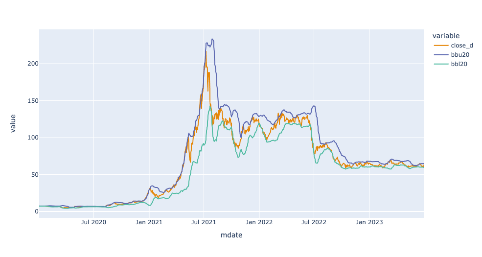
tejapi.ApiConfig.ignoretz = True
For the period from 2021–06–01 to 2022–12–31, we take YangMing Marine Transport Corporation(2609) as an example, we will use unadjusted closed price、BB-Upper(20)、BB-Lower(20) to construct the Bollinger Band, and then we will compare the return with Market Return Index(Y9997)
stock_id = "2609"
gte, lte = '2020-01-01', '2023-06-30'
stock = tejapi.get('TWN/APRCD',
paginate = True,
coid = stock_id,
mdate = {'gte':gte, 'lte':lte},
opts = {
'columns':[ 'mdate', 'open_d', 'high_d', 'low_d', 'close_d', 'volume']
}
)
ta = tejapi.get('TWN/AVIEW1',
paginate = True,
coid = stock_id,
mdate = {'gte':gte, 'lte':lte},
opts = {
'columns':[ 'mdate', 'bbu20', 'bbma20', 'bbl20']
}
)
market = tejapi.get('TWN/APRCD',
paginate = True,
coid = "Y9997",
mdate = {'gte':gte, 'lte':lte},
opts = {
'columns':[ 'mdate', 'close_d', 'volume']
}
)
data = stock.merge(ta, on = ['mdate'])
market.columns = ['mdate', 'close_m', 'volume_m']
data = data.set_index('mdate')
After acquiring the stock price and technical indicators data, as in the previous article, we use plotly.express to visualize our Bollinger Band. In the diagram, bbu20 will be the upper track 、bbl20 will be the lower track, and close_d will be the closed price.
fig = px.line(data,
x=data.index,
y=["close_d","bbu20","bbl20"],
color_discrete_sequence = px.colors.qualitative.Vivid
)
fig.show()
Next, we will implement two Bollinger Band trading strategies and compare their differences.
In light of the only difference in strategies is the transaction’s unit price, we modify our strategy code in the previous article. We define our strategy in def bollingeband_strategy, add an if condition, and set a parameter — mode to control which strategy we want to execute. When mode is True, execute strategy 1; when mode is False, run strategy 2.
def bollingeband_strategy(data, principal, cash, position, order_unit, mode):
trade_book = pd.DataFrame()
for i in range(data.shape[0] -2):
cu_time = data.index[i]
cu_close = data.loc[cu_time, 'close_d']
cu_bbl, cu_bbu = data.loc[cu_time, 'bbl20'], data.loc[cu_time, 'bbu20']
if mode:
n_time = data.index[i + 1]
n_open = data['open_d'][i + 1]
else:
n_time = data.index[i]
n_open = data['close_d'][i]
if position == 0: #進場條件
if cu_close <= cu_bbl and cash >= n_open*1000:
position += 1
order_time = n_time
order_price = n_open
order_unit = 1
friction_cost = (20 if order_price*1000*0.001425 < 20 else order_price*1000*0.001425)
total_cost = -1 * order_price * 1000 - friction_cost
cash += total_cost
trade_book = pd.concat([trade_book,
pd.DataFrame([stock_id, 'Buy', order_time, 0, total_cost, order_unit, position, cash])],
ignore_index = True, axis=1)
elif position > 0:
if cu_close >= cu_bbu: # 出場條件
order_unit = position
position = 0
cover_time = n_time
cover_price = n_open
friction_cost = (20 if cover_price*order_unit*1000*0.001425 < 20 else cover_price*order_unit*1000*0.001425) + cover_price*order_unit*1000*0.003
total_cost = cover_price*order_unit*1000-friction_cost
cash += total_cost
trade_book = pd.concat([trade_book,
pd.DataFrame([stock_id, 'Sell', 0, cover_time, total_cost, -1*order_unit, position, cash])],
ignore_index = True, axis=1)
elif cu_close <= cu_bbl and cu_close <= order_price and cash >= n_open*1000: #加碼條件: 碰到下界,比過去買入價格貴
order_unit = 1
order_time = n_time
order_price = n_open
position += 1
friction_cost = (20 if order_price*1000*0.001425 < 20 else order_price*1000*0.001425)
total_cost = -1 * order_price * 1000 - friction_cost
cash += total_cost
trade_book = pd.concat([trade_book,
pd.DataFrame([stock_id, 'Buy', order_time, 0, total_cost, order_unit, position, cash])],
ignore_index = True, axis=1)
if position > 0: # 最後一天平倉
order_unit = position
position = 0
cover_price = data['open_d'][-1]
cover_time = data.index[-1]
friction_cost = (20 if cover_price*order_unit*1000*0.001425 < 20 else cover_price*order_unit*1000*0.001425) + cover_price*order_unit*1000*0.003
cash += cover_price*order_unit*1000-friction_cost
trade_book = pd.concat([trade_book,
pd.DataFrame([stock_id, 'Sell',0,cover_time, cover_price*order_unit*1000-friction_cost, -1*order_unit, position, cash])],ignore_index=True, axis=1)
trade_book = trade_book.T
trade_book.columns = ['Coid', 'BuyOrSell', 'BuyTime', 'SellTime', 'CashFlow','TradeUnit', 'HoldingPosition', 'CashValue']
return trade_book
Now we build an automated trading strategy. The return of the def bollingeband_strategy is a transaction table that could let us understand each transaction’s details. Further, we define a def simplify to summarize all info for better readability.
def simplify(trade_book):
trade_book_ = trade_book.copy()
trade_book_['mdate'] = [trade_book.BuyTime[i] if trade_book.BuyTime[i] != 0 else trade_book.SellTime[i] for i in trade_book.index]
trade_book_ = trade_book_.loc[:, ['BuyOrSell', 'CashFlow', 'TradeUnit', 'HoldingPosition', 'CashValue' ,'mdate']]
return trade_book_
The final step is calculating both strategies’ performance. Basically, the code in this part is similar to the previous code. However, because of the upgrade of the pandas version, the latest version no longer supports the function append; we made a slight modification to make the code can keep working and wrap it in def back_test.
def back_test(principal, trade_book_, data, market):
cash = principal
data_ = data.copy()
data_ = data_.merge(trade_book_, on = 'mdate', how = 'outer').set_index('mdate')
data_ = data_.merge(market, on = 'mdate', how = 'inner').set_index('mdate')
# fillna after merge
data_['CashValue'].fillna(method = 'ffill', inplace=True)
data_['CashValue'].fillna(cash, inplace = True)
data_['TradeUnit'].fillna(0, inplace = True)
data_['HoldingPosition'] = data_['TradeUnit'].cumsum()
# Calc strategy value and return
data_["StockValue"] = [data_['open_d'][i] * data_['HoldingPosition'][i] *1000 for i in range(len(data_.index))]
data_['TotalValue'] = data_['CashValue'] + data_['StockValue']
data_['DailyValueChange'] = np.log(data_['TotalValue']) - np.log(data_['TotalValue']).shift(1)
data_['AccDailyReturn'] = (data_['TotalValue']/cash - 1) *100
# Calc BuyHold return
data_['AccBHReturn'] = (data_['open_d']/data_['open_d'][0] -1) * 100
# Calc market return
data_['AccMarketReturn'] = (data_['close_m'] / data_['close_m'][0] - 1) *100
# Calc numerical output
overallreturn = round((data_['TotalValue'][-1] / cash - 1) *100, 4) # 總績效
num_buy, num_sell = len([i for i in data_.BuyOrSell if i == "Buy"]), len([i for i in data_.BuyOrSell if i == "Sell"]) # 買入次數與賣出次數
num_trade = num_buy #交易次數
avg_hold_period, avg_return = [], []
tmp_period, tmp_return = [], []
for i in range(len(trade_book_['mdate'])):
if trade_book_['BuyOrSell'][i] == 'Buy':
tmp_period.append(trade_book_["mdate"][i])
tmp_return.append(trade_book_['CashFlow'][i])
else:
sell_date = trade_book_["mdate"][i]
sell_price = trade_book_['CashFlow'][i] / len(tmp_return)
avg_hold_period += [sell_date - j for j in tmp_period]
avg_return += [ abs(sell_price/j) -1 for j in tmp_return]
tmp_period, tmp_return = [], []
avg_hold_period_, avg_return_ = np.mean(avg_hold_period), round(np.mean(avg_return) * 100,4) #平均持有期間,平均報酬
max_win, max_loss = round(max(avg_return)*100, 4) , round(min(avg_return)*100, 4) # 最大獲利報酬,最大損失報酬
winning_rate = round(len([i for i in avg_return if i > 0]) / len(avg_return) *100, 4)#勝率
min_cash = round(min(data_['CashValue']),4) #最小現金持有量
print('總績效:', overallreturn, '%')
print('交易次數:', num_trade, '次')
print('買入次數:', num_buy, '次')
print('賣出次數:', num_sell, '次')
print('平均交易報酬:', avg_return_, '%')
print('平均持有期間:', avg_hold_period_ )
print('勝率:', winning_rate, '%' )
print('最大獲利交易報酬:', max_win, '%')
print('最大損失交易報酬:', max_loss, '%')
print('最低現金持有量:', min_cash)
So far, we already finished the whole coding process, then we can compare both strategies’ performance with real data.
Trade at the open price of tomorrow
principal = 500000
cash = principal
position = 0
order_unit = 0
trade_book = bollingeband_strategy(data, principal, cash, position, order_unit, True)
trade_book_ = simplify(trade_book)
back_test(principal, trade_book_, data, market)
Trade at the closed price of today
principal = 500000
cash = principal
position = 0
order_unit = 0
trade_book_cu_close = bollingeband_strategy(data, principal, cash, position, order_unit, False)
trade_book_cu_close_ = simplify(trade_book_cu_close)
back_test(principal, trade_book_cu_close_, data, market)
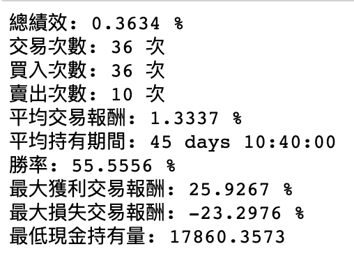
By observing the results of two trading strategies, it can be noticed that trading based on the day’s closing price yields better overall performance. However, novice stock market participants may mistakenly use the historical backtesting data and assume the closing price as the trading price, disregarding the fact that it is impossible to know the closing price in advance in the actual market. Using information that is not known when trading for backtesting constitutes a “look-ahead bias,” resulting in discrepancies in the backtesting results. Therefore, it is advisable to use the next day’s opening price as the trading price to reflect the most accurate trading conditions.
Through this implementation of simple trading backtest, we have demonstrated the presence of the look-ahead bias in backtesting, which is not limited to trading alone but is a common occurrence in the field of finance. In order to avoid the look-ahead bias, it is crucial to ensure that historical analysis or decision-making processes are based solely on the information available at that time. This requires using historical data in a manner consistent with what was known in the past, excluding any subsequent information that was not available at the time. Being aware of the look-ahead bias and handling the data with caution is essential for maintaining the integrity and accuracy of statistical analysis and decision-making processes.
Last but not least, please note that the “Stocks this article mentions are just for discussion. Please do not consider it to be any recommendations or suggestions for investment or products.” Hence, if you are interested in issues like Creating Trading Strategy, Performance Backtesting, and Evidence-based research, you are welcome to purchase the plans offered in TEJ E-Shop and use the well-complete database to create your optimal trading strategy.