Table of Contents
The Williams %R is also called the Williams index, wmsr, or W%R. It was created by the famous American trader Larry Williams in 1973. It is a standard indicator in technical analysis.
The William indicator is the earliest indicator to judge whether the market price is overbought or oversold. The KD line and other indicators commonly used by investors to judge overbought or oversold are developed based on the William indicator.
The Williams %R is calculated as follows:
According to the above formula, it can be known that the value of the Williams %R ranges from 0 to -100. When the indicator’s value is between 0 and -50, the stock price is in a strong stage; when the indicator’s value falls between -51 and -100, the stock price is in a weak stage. In addition, when the indicator value is less than -80, it means that the stock price may be in an oversold state, which is a good time to buy; and when the indicator value is greater than -20, it means that the stock price may be in an overbought state, and it is a good time to sell.
In addition, the time parameters of the Williams %R have a considerable impact on it, so investors need to set parameters that suit them according to their habits.
This article uses the Williams %R to determine the timing of overbought and oversold stocks. It uses the following entry and exit rules to establish a trading strategy and perform backtesting:
Buy the stock when the Williams %R ≤ -80 because the market is too cold and the stock is in the oversold stage.
When the Williams %R ≥ -20, sell the stock because the market is overheated and the stock is in the overbought stage.
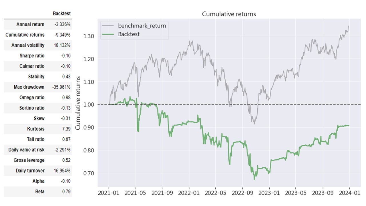
In addition, this article sets the N value to 100 days instead of the more common pane used in calculating the Williams %R. Finally, the 14 days often used in the industry will be used for backtest comparison.
This article uses Windows 11 and Jupyter Notebook as the editor.
This strategy lasts for three years, from 2021-01-01 to 2023-12-31, focusing on electronics stocks: Hon Hai Precision (2317), Yageo (2327), TSMC (2330), Acer (2353), Asus (2357), and Quanta (2382) are used as examples, and the return index (IR0001) is used as the broader market for performance comparison.
import os
os.environ['TEJAPI_KEY'] = "your key"
os.environ['TEJAPI_BASE'] = "https://api.tej.com.tw"
import pandas as pd
import numpy as np
import matplotlib.pyplot as plt

from zipline.data import bundles
from zipline.utils.calendar_utils import get_calendar
from zipline.sources.TEJ_Api_Data import get_Benchmark_Return

start = '2021-01-01'
end = '2023-12-31'

os.environ['ticker'] = 'IR0001 2317 2327 2330 2353 2357 2382'
os.environ['mdate'] = start+' '+end
!zipline ingest -b tquantCustomFactor allows users to design the required customization factors. In this case, we use it to handle:
from zipline.data import bundles
from zipline.sources.TEJ_Api_Data import get_Benchmark_Return
from zipline.pipeline.mixins import SingleInputMixin
from zipline.pipeline.data import TWEquityPricing
from zipline.pipeline.factors import CustomFactor
from zipline.pipeline import Pipeline
from zipline.TQresearch.tej_pipeline import run_pipeline
from zipline.pipeline.filters import StaticAssets
from zipline.utils.math_utils import nanmax, nanmin

class Wmsr(CustomFactor):
    inputs = [TWEquityPricing.close, TWEquityPricing.high, TWEquityPricing.low]
    window_length = 100

    def compute(self, today, assets, out, close, high, low):
        highest_highs = nanmax(high, axis=0)
        lowest_lows = nanmin(low, axis=0)
        williams_index = ((highest_highs - close[-1]) / (highest_highs - lowest_lows)) * 100 * -1

        out[:] = williams_index
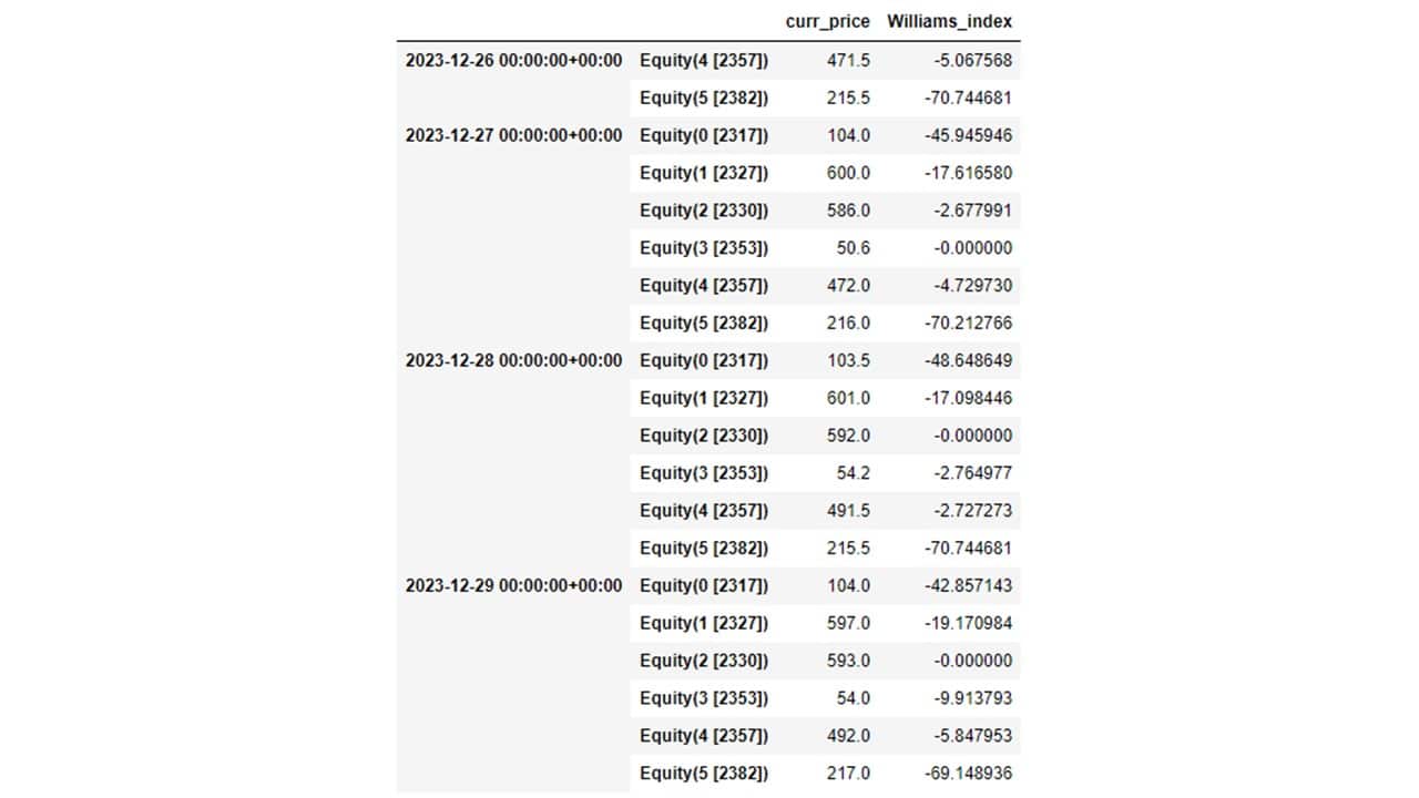
Pipeline() provides users with the function of quickly processing multiple targets’ quantitative indicators and price and volume data. In this case, we use it to process:
The current stock price of the stock (curr_price)
start_dt, end_dt = pd.Timestamp(start, tz='utc'), pd.Timestamp(end, tz='utc')
bundle = bundles.load('tquant')
benchmark_asset = bundle.asset_finder.lookup_symbol('IR0001',as_of_date = None)

def make_pipeline():
    wmsr = Wmsr()
    curr_price = TWEquityPricing.close.latest

    return Pipeline(
        columns = {
            'curr_price':curr_price,
            'Williams_index' : wmsr,
        },
        screen = ~StaticAssets([benchmark_asset])
    )
my_pipeline = run_pipeline(make_pipeline(),start_dt, end_dt)
my_pipeline.tail(20)
The initialize() function is used to define the daily trading environment before the start of trading. In this example, we set:
from zipline.finance import slippage, commission
from zipline.api import *
from zipline.api import set_slippage, set_commission, set_benchmark, attach_pipeline, order, order_target, symbol, pipeline_output, record

def initialize(context):
    set_slippage(slippage.VolumeShareSlippage(volume_limit = 0.025, price_impact = 0.1))
    set_commission(commission.Custom_TW_Commission(min_trade_cost = 20, discount = 1.0, tax = 0.003))
    attach_pipeline(make_pipeline(), 'mystrats')
set_benchmark(symbol('IR0001'))The handle_data() function is important for constructing the Williams %R strategy. It is called every day after the start of backtesting, and its main tasks include setting trading strategies, placing orders, and recording trading information.
def handle_data(context, data):
    out_dir = pipeline_output('mystrats')

    for i in out_dir.index:
        curr_price = out_dir.loc[i, 'curr_price']
        w_value = out_dir.loc[i, 'Williams_index']
        stock_position = context.portfolio.positions[i].amount
        cash_position = context.portfolio.cash

        if stock_position == 0 and cash_position >= curr_price * 1000:
            if w_value <= -80:
                order(i, 1000)
        elif stock_position > 0:
            if w_value <= -80 and cash_position >= curr_price * 1000:
                order(i, 1000)

            elif w_value >= -20:
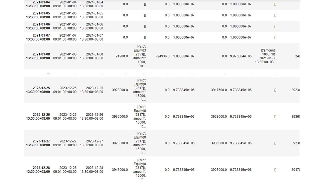
order_target(i, 0)Use the run_algorithm() function to execute the Williams %R strategy as defined above. Set the trading period from start_dt (2021-01-01) to end_dt (2023-12-31), using the dataset tquant, with an initial capital of 20 million dollars. The output results represent the daily performance and trade details.
from zipline import run_algorithm

start_date = pd.Timestamp('2021-01-01',tz='utc')
end_date = pd.Timestamp('2023-12-31',tz='utc')

results = run_algorithm(start = start_date,
                        end = end_date,
                        initialize = initialize,
                        capital_base = 1e7,
                        handle_data = handle_data,
                        data_frequency = 'daily',
                        bundle = 'tquant'
                        )
results
import pyfolio as pf
from pyfolio.utils import extract_rets_pos_txn_from_zipline

returns, positions, transactions = pf.utils.extract_rets_pos_txn_from_zipline(results)
benchmark_rets = results.benchmark_return

# Creating a Full Tear Sheet
pf.create_full_tear_sheet(returns, positions = positions, transactions = transactions,
                          benchmark_rets = benchmark_rets,
                          round_trips=False)
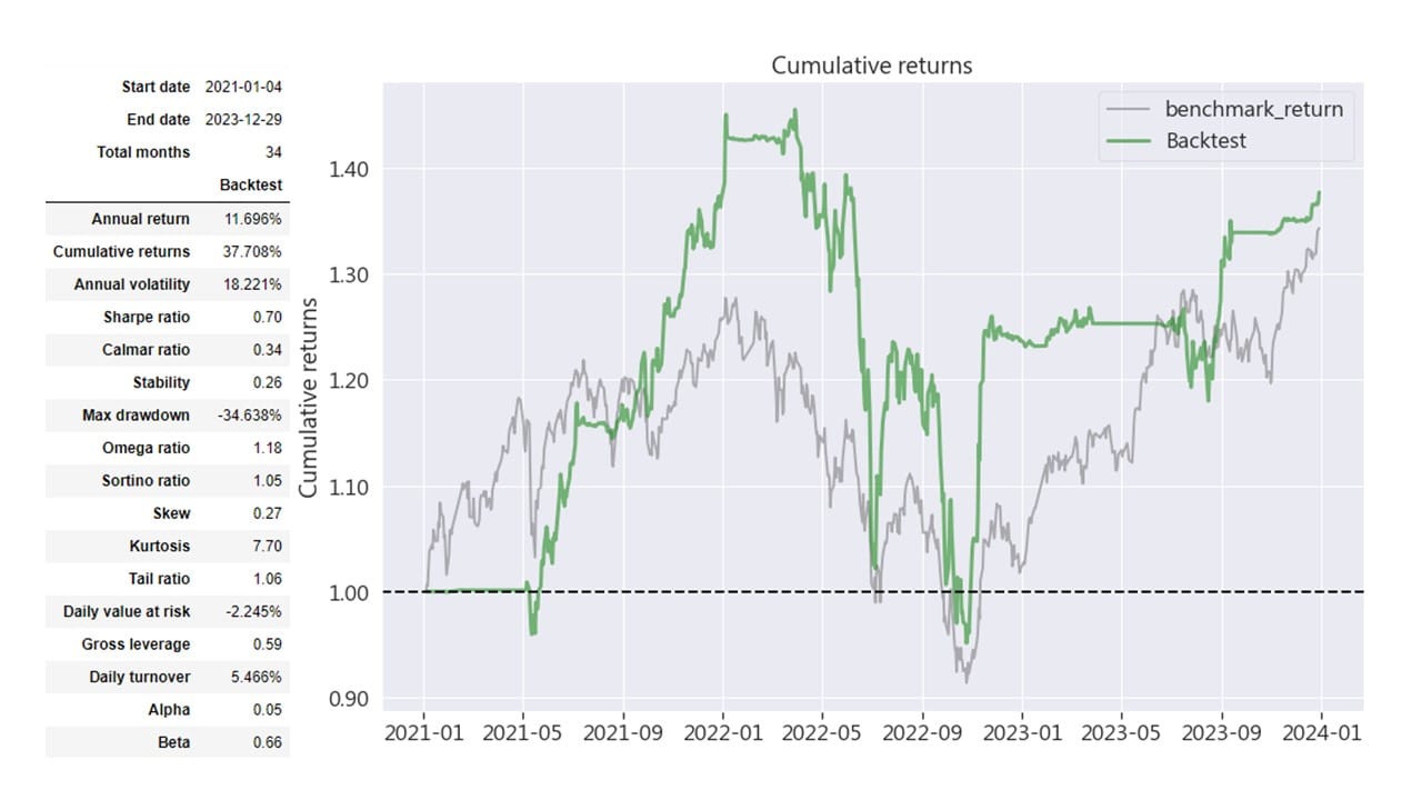
In these 34 months, the Williams %R strategy obtained an annualized return of 11.696%, with a cumulative return of 37.708%. The profit performance was generally slightly better than the market; however, the annualized volatility and maximum drawdown were 18.221% and -34.638% respectively, showing that the risk of market fluctuations using the Williams %R strategy is more significant. When used, because the fluctuations are too large, it is impossible to rely solely on the Williams %R for quantitative trading. It can be combined with the TQuant Lab Ichimoku Kinko Hyo Strategy, A Self-contained Technical Analysis Indicator in the previous article, a set of self-contained technical analysis indicators such as the moving index loss or the moving average. The method matches the Williams %R to increase the stability of investment.

This chart only changes the time parameter and shows that the Williams %R time parameter has a huge impact. Since the Williams %R is more sensitive to price than other technical indicators, if you only follow the fast-line (short-day) Williams %R, buying and selling may be performed too frequently, leading to misjudgments.
This strategy uses the Williams %R to conduct backtest simulations, using the indicator to enter the market when it is oversold and exit when it is overbought. The backtest results show that investors sometimes get more rewards compared to the broader market, but investors will bear the excessive market pressure. Fluctuation risk and time parameters have a huge impact on indicators. Therefore, investors must pay attention to their habits and adjust them to suitable parameters when investing. Also, note that the Williams %R is only a technical indicator and should be combined with other auxiliary judgments when investing to increase the stability and reliability of the investment.
In the future, I will continue to introduce various indicators constructed using the TEJ database and backtest their performance. Therefore, readers interested in trading backtests are encouraged to explore TQuant Lab‘s related solutions, utilizing high-quality databases to build their trading strategies.
A friendly reminder: This strategy is for reference only and does not constitute any recommendation for commodities or investments.
[TQuant Lab] Solving Your Quantitative Finance Pain Points
Comprehensively providing all the tools needed for trading backtesting.