
In the 1970s, Eugene Fama introduced the Efficient-market Hypothesis (EMH). The hypothesis assumes that individuals act as rational economic beings who objectively consider all relevant information to make ration decisions. And therefore, the stock price is reasonably estimated by investors and maintains at its “equilibrium price.” However, in the 1980s, anomalies that could not be explained by the EMH appeared one after another, indicating that the stock price would deviate from its equilibrium price. Observing these phenomena, Behavioral Finance believed that investors were irrational. The irrationality caused the stock price to be erroneously estimated by investors, and thus deviate from its equilibrium price, resulting in “mispricing.”
Table of Contents
From the above, if we can successfully catch the so-called mispricing, we can profit from it. The concept sounds easy, but the implementation is never the case. Because we don’t know the true equilibrium price of the stock, it is difficult to observe the degree of mispricing or mispricing itself. In order to solve this problem, some scholars propose different means of estimating mispricing. For instance, Brennan and Wang (2010) proposed Mispricing Return Premium. They used companies listed on NYSE, AMEX, and NASDAQ from 1962 to 2007 as samples, and estimated the mispricing based on two assumptions which were Fama-French (1993) three-factor model and the AR(1) process. They adopted the Kalman filter to estimate the mispricing factor and used it to construct an investment strategy. The model found that using this strategy in the US stock market could obtain a return rate as high as about 35% in a year, which confirmed the effectiveness mispricing factor generating abnormal returns.
According to the mispricing method above, first, it is assumed that the fundamental return, R*, can be represented by Fama-French three-factor model:

R*(i,t) is the fundamental return of each stock i per month t, Rf is the risk-free interest rate, R(M,t), SMBt, HMLt are Fama-French factors, and ϵ(i,t) is the theoretical residual rate of return. It means that, ideally, all stock returns in the market can be explained by market factors, size factors and book-to-price ratio factors. The actual return R (market return) can be explained by the following model:

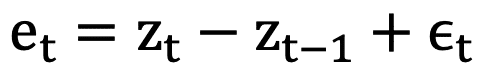
R(i,t) is the actual return of stock i per month t, ai is the mispricing premium, and e(i,t) is the actual residual rate of return. It means that in reality, stock returns may have other risks that cannot be explained by the three factors, that is, the theoretical residuals actually contain mispricing premiums. Meanwhile, 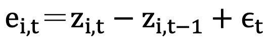 , the actual residual in this period is the theoretical residual plus the degree of deviation of the stock price in the two periods.Next, in order to obtain the mispricing factor zt, we refer to the estimation of Khil and Lee (2002), whose Kalman filter observation equation was:
Referring to the research of Potterba and Summers (1988), we assume that the mispricing corresponds with the AR(1) process, that is, the mispricing factor of this period is correlated with the mispricing factor of the previous period. The assumption is further applied to the Kalman filter state equation
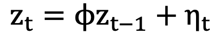
Therefore, with the observation equation based on the Fama-French three-factor model and the state equation based on the AR(1) process, the mispricing factor z_(i,t) can be estimated using the Kalman filter.
Table 1: Performance Analysis of Mispricing Factors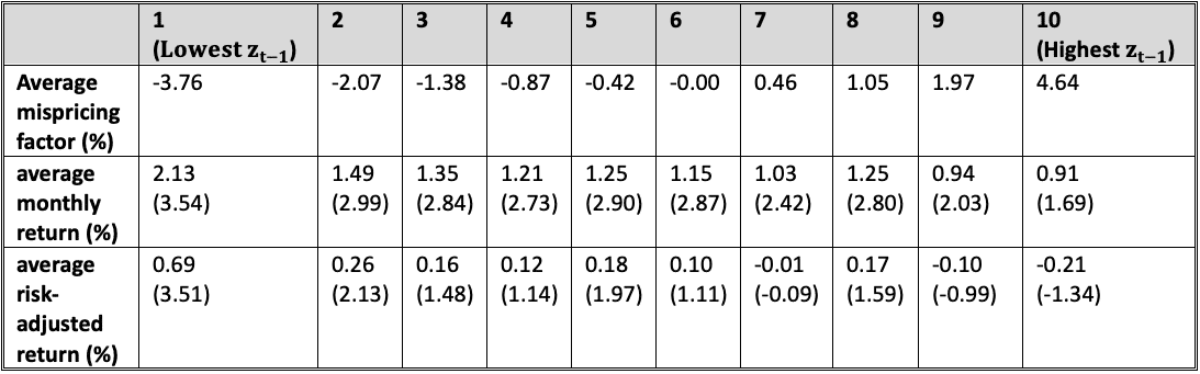
Note: The numbers in parentheses are t statistics
The Relationship Between the Degree of Mispricing and ReturnTable 1 shows that the stocks are arranged according to the mispricing factor from lowest to highest and divided into ten groups. Holding stocks in the higher groups should lead to better returns given the greater degree of mispricing. To test this assumption, consider holding a portfolio of stocks in the top 2, 2.5, and 5 quantiles and observe how this strategy performs with greater mispricing. The results are shown in Table 2. The greater the degree of mispricing, the better the rate of return the mispricing strategy can generate.
Table 2: Performance of Holding Portfolios of Stocks with Different Quantiles
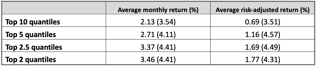
Note: The numbers in parentheses are t statistics
The Relationship Between Investment Holding Period and Return
Does the holding period affect the reward? Figure 1 shows the cumulative rate of return of the lowest group of mispricing factors under different holding periods. It can be found that the longer the holding periods, the more information stock price reflects, and the price gradually returns to equilibrium.
Figure 1: Cumulative Rate of Return (%) under Different Holding Periods
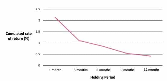
Table 3 shows the annualized rate of return under different holding periods. It can be found that using the mispricing strategy to hold for one month has the best return.
Table 3: Performance of Different Holding Periods
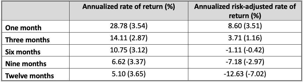
Note: The numbers in parentheses are t statistics
Using the Kalman filter of Brennan and Wang (2010) and conducting empirical research on the Taiwan market from 2000 to 2019, we discovered the effectiveness of mispricing generating excess returns. And if you implement this strategy in Taiwan stocks, you would be expected to get an annualized rate of return of about 29% in one year.
Next, the results showed that holding the stock portfolio in the top 2 quantiles would get the highest annualized return of 50.41%. The higher the degree of mispricing, the better the return on the mispricing strategy. In addition, the highest cumulative return occurs when the holding period is one month, and the strategy would have no material effect after the holding period exceeds one month.
Taken together, we demonstrate that mispricing strategies could pay off well. Investors could use the mispricing factor to build strategies and expect to earn returns in the Taiwan stock market.
