Table of Contents
追逐利益、趨避風險是投資人的目標,預測股價動是達成上述目標的方法之一。過去人們使用ARIMA、GARCH等時間序列,試圖刻畫出未來股價的軌跡。到了今日,隨著深度學習的蓬勃發展,越來越多時間序列相關的模型的出現,似乎能應用於未來股價的預測中。本文即是利用GRU與LSTM兩序列相關模型進行股價預測,使用前5日的開盤、最高、最低、收盤價預測隔日收盤價。
過去【資料科學】LSTM已對LSTM有相當程度的介紹,於此不在多做贅述。本文多加入了同樣是RNN家族的GRU模型,檢驗GRU與LSTM在股價預測上的表現差異。GRU改動了LSTM中記憶單元的遺忘、輸入與輸出門,將其縮編為更新門與重置門,前者類似於LSTM中的遺忘與輸入門,負責決定每次迭代需保留與丟棄的信息,後者則是決定需丟棄過去累積的信息。從三門減少至雙門的情況下,GRU相較於LSTM能達成較快的運算速度,且其表現理論上不亞於LSTM。
本文使用Google Colab作為編輯器
# 載入所需套件
import pandas as pd
import numpy as np
from sklearn.preprocessing import StandardScaler
import plotly.graph_objects as go
import os
import time
import tejapi
import math
import torch
from torch import nn, optim
from torch.utils.data import Dataset, DataLoader, TensorDataset

# 登入TEJ API
api_key = 'YOUR_KEY'
tejapi.ApiConfig.api_key = api_key
tejapi.ApiConfig.ignoretz = True

# 載入gpu
device = torch.device('cuda' if torch.cuda.is_available() else 'cpu')
公司交易面資料庫: 未調整股價(日),資料代碼為(TWN/APRCD)。
使用台積電(2330.tw)未調整開盤、最高、最低與收盤價格,時間區間為2019/01/01到2023/01/01。先依照8:2進行訓練與驗證集切分,再進行標準化。標準化能有效減少特徵規模大小不均所造成的偏誤且能加速訓練時間。
# 股價
gte, lte = '2019-01-01', '2023-01-01'
data = tejapi.get('TWN/APRCD',
                   paginate = True,
                   coid = '2330',
                   mdate = {'gte':gte, 'lte':lte},
                   opts = {
                       'columns':[ 'mdate', 'open_d', 'high_d', 'low_d', 'close_d', 'volume']
                   }
                  )

train_size = int(0.8 * len(data))
train, test = data.iloc[:train_size, :4], data.iloc[train_size:, :4]

scaler_train = StandardScaler()
train = scaler_train.fit_transform(train)

scaler_test = StandardScaler()
test = scaler_test.fit_transform(test)
建立Pytorch Dataset與DataLoader,可以自動建置Batch以方便後續將資料餵給模型訓練。
def create_dataset(dataset, lookback):
    X, y = [], []
    for i in range(len(dataset)-lookback):
        feature = dataset[i:i+lookback, :]
        target = dataset[i+1:i+lookback+1][-1][-1]
        X.append(feature)
        y.append(target)
    return torch.FloatTensor(X).to(device), torch.FloatTensor(y).view(-1, 1).to(device)

lookback = 5
X_train, y_train = create_dataset(train, lookback = lookback)
X_val, y_val = create_dataset(test, lookback = lookback)
print(X_train.size(), y_train.size())
print(X_val.size(), y_val.size())
loader = DataLoader(TensorDataset(X_train, y_train), shuffle = False, batch_size = 32)
模型架構為一層LSTM,加上一層Dropout後,再接上一個全連接層。加入Dropout的原因為防止模型產生過擬合問題。
● input_size: 為輸入的特徵數量,使用開盤、最高、最低與收盤價格,故 input_size = 4。
● hidden_size: 為LSTM隱藏層神經元數。
● num_layer: LSTM層數,單層預設為一。
● batch_first: 輸出維度保持(batch_size, sequence_len, hidden_size),其中 sequence_len為5,因為我們採用五天價格預測隔日價格。
# 建立單層LSTM函式
class S_LSTM(nn.Module):
    def __init__(self):
        super().__init__()
        self.lstm1 = nn.LSTM(input_size = 4, hidden_size=64, num_layers=1, batch_first=True)
        self.dropout = nn.Dropout(0.2)
        self.linear = nn.Linear(64, 1)
    def forward(self, x):
        x, _ = self.lstm1(x)
        x = self.dropout(x)
        x = x[:, -1, :]
        x = self.linear(x)
        return x
#載入訓練模型
def trainer(epochs, loader, X_train, y_train, X_val, y_val, model, criterion, optimizer):
    train_loss, test_loss = [], []
    best_rmse = float('inf')
    best_y_true, best_y_pred = None, None
    best_model_state = None
    best_epoch = -1  # 記錄最佳 Epoch

    for epoch in range(epochs):
        model.train()
        for batch, (x, y_true) in enumerate(loader):
            y_pred = model(x)
            loss = criterion(y_pred, y_true)
            loss.backward()
            optimizer.step()
            optimizer.zero_grad()

        model.eval()
        with torch.no_grad():
            y_pred_val = model(X_train)
            train_rmse = np.sqrt(criterion(y_pred_val, y_train).item())
            train_loss.append(train_rmse)
            y_pred_val = model(X_val)
            test_rmse = np.sqrt(criterion(y_pred_val, y_val).item())
            test_loss.append(test_rmse)

            # 儲存最佳結果
            if test_rmse < best_rmse:
                best_rmse = test_rmse
                best_y_true = y_val.cpu().numpy()
                best_y_pred = y_pred_val.cpu().numpy()
                best_model_state = model.state_dict()
                best_epoch = epoch + 1  # 記錄最佳 Epoch

    # 載入最佳模型權重
    model.load_state_dict(best_model_state)
    return train_loss, test_loss, best_y_true, best_y_pred, best_epoch
# 設置模型、損失函數與優化器
model = S_LSTM().to(device)
criterion = nn.MSELoss()
optimizer = optim.Adam(model.parameters())
epochs = 1000


#紀錄訓練時間
start = time.time()
slstm_train_loss, slstm_test_loss, slstm_y_true, slstm_y_pred, slstm_best_epoch = trainer(
    epochs, loader, X_train, y_train, X_val, y_val, model, criterion, optimizer
)
end = time.time()
print('single lstm time cost %.4f' %(end-start))
fig = go.Figure()
fig.add_trace(go.Scatter(x=np.arange(epochs), y=slstm_train_loss,
                    mode='lines',
                    name='Train Loss'))
fig.add_trace(go.Scatter(x=np.arange(epochs) , y=slstm_test_loss,
                    mode='lines',
                    name='Validation Loss'))
fig.update_layout(
    title="Loss curve for single lstm",
    xaxis_title="epochs",
    yaxis_title="rmse"
)
fig.show()
從損失曲線圖可以觀察到,在訓練過程中,訓練集的損失迅速下降,並於約第100次 epoch 之後趨於穩定,最終損失值接近於 0.05 左右。而驗證集的損失也在大約第150次 epoch 後趨於穩定,並維持在 0.2 左右的範圍。後續再將股價預測圖繪製檢驗模型的預測能力。
train_plot = np.ones_like(data[:, 3]) * np.nan
test_plot = np.ones_like(data[:, 3]) * np.nan
with torch.no_grad():
  # 預測訓練集資料
  y_pred = model(X_train)
  train_plot[lookback:int(0.8 * len(data))] = y_pred.view(-1).cpu()
  # 預測驗證集資料
  y_pred = model(X_val)
  test_plot[int(0.8 * len(data))+lookback:] = y_pred.view(-1).cpu()

fig = go.Figure()
fig.add_trace(go.Scatter(x=mdate, y=train_plot,
                    mode='lines',
                    name='Train'))
fig.add_trace(go.Scatter(x=mdate , y=test_plot,
                    mode='lines',
                    name='Validation'))
fig.add_trace(go.Scatter(x=mdate , y=data[:, 3],
                    mode='lines',
                    name='True'))
fig.update_layout(
    title="Stock prediction for sngle lstm",
    xaxis_title="dates",
    yaxis_title="standardised stock"
)
fig.show()
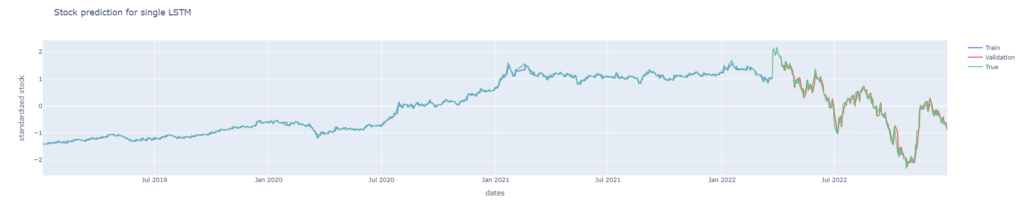
從上圖與損失曲線圖可以發現單層LSTM對於股價的預測能力是相當不錯的。這點十分有趣,因為根據【資料科學】LSTM所述,他們在單層的LSTM表現是較差的,並無法完整捕捉到時間序列資訊。而我們與他們的區別在於他們有多採用每日成交量作為輸入資料的特徵、我們的LSTM層輸出維度是64而他們的是32,Dropout的比率我們是20%而他們的是30%。目前認為最有可能造成差異的原因應該為他們多採用了每日成交量作為輸入特徵。
雖然單層LSTM已經可以達成不錯的效果,但我們不彷多堆疊幾層LSTM去試看看是否能繼續最佳化。多層LSTM的架構為: 一層LSTM + 一層Dropout + 一層LSTM + 一層Dropout + 一層全連接層。其中兩次Dropout的比率都調整為40%,這裡將比率調高的原因是為了避免過擬合問題。
# 建立雙層LSTM函式
class LSTM(nn.Module):
    def __init__(self):
        super().__init__()
        self.lstm1 = nn.LSTM(input_size = 4, hidden_size=64, num_layers=1, batch_first=True)
        self.dropout1 = nn.Dropout(0.4)
        self.lstm2 = nn.LSTM(input_size = 64, hidden_size=32, num_layers=1, batch_first=True)
        self.dropout2 = nn.Dropout(0.4)
        self.linear = nn.Linear(32, 1)
    def forward(self, x):
        x, _ = self.lstm1(x)
        x = self.dropout1(x)
        x, _ = self.lstm2(x)
        x = self.dropout2(x)
        x = x[:, -1, :]
        x = self.linear(x)
        return x
#載入訓練模型
def trainer(epochs, loader, X_train, y_train, X_val, y_val, model, criterion, optimizer):
    train_loss, test_loss = [], []
    best_rmse = float('inf')
    best_y_true, best_y_pred = None, None
    best_model_state = None
    best_epoch = -1  # 記錄最佳 Epoch

    for epoch in range(epochs):
        model.train()
        for batch, (x, y_true) in enumerate(loader):
            y_pred = model(x)
            loss = criterion(y_pred, y_true)
            loss.backward()
            optimizer.step()
            optimizer.zero_grad()

        model.eval()
        with torch.no_grad():
            y_pred_val = model(X_train)
            train_rmse = np.sqrt(criterion(y_pred_val, y_train).item())
            train_loss.append(train_rmse)
            y_pred_val = model(X_val)
            test_rmse = np.sqrt(criterion(y_pred_val, y_val).item())
            test_loss.append(test_rmse)

            # 儲存最佳結果
            if test_rmse < best_rmse:
                best_rmse = test_rmse
                best_y_true = y_val.cpu().numpy()
                best_y_pred = y_pred_val.cpu().numpy()
                best_model_state = model.state_dict()
                best_epoch = epoch + 1  # 記錄最佳 Epoch

    # 載入最佳模型權重
    model.load_state_dict(best_model_state)
    return train_loss, test_loss, best_y_true, best_y_pred, best_epoch
# 設置模型、損失函數與優化器
model = LSTM().to(device)
criterion = nn.MSELoss()
optimizer = optim.Adam(model.parameters())
epochs = 1000
# 開始訓練並且計算訓練所需時間
start = time.time()
lstm_train_loss, lstm_test_loss, lstm_y_true, lstm_y_pred, lstm_best_epoch = trainer(epochs, loader, X_train, y_train, X_val, y_val, model, criterion, optimizer)end = time.time()
print('stack lstm time cost %.4f' %(end-start))
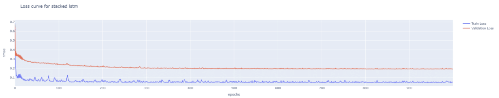
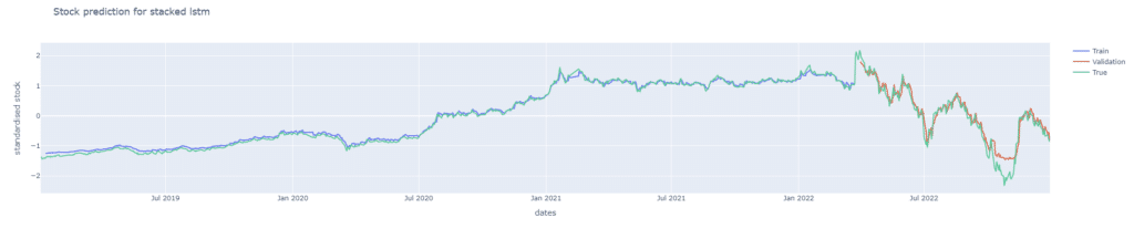
從雙層 LSTM 的損失曲線可以發現,隨著模型複雜度的提升,其損失下降的速度相較單層 LSTM 更加緩慢,在驗證集上逐漸穩定,最終大約收斂至 0.08 左右。同時可以觀察到,雙層 LSTM 的驗證損失在訓練過程中稍高於訓練損失,顯示模型在泛化能力上有一定的挑戰。後續再將股價預測圖繪製檢驗模型的預測能力,可以發現預測能力較不如單層LSTM,但也能抓出漲跌趨勢。
接著我們使用GRU模型預測股價,一樣先加上一層GRU層,在疊上一層比率為0.2的Dropout跟全連接層。
# 建立單層GRU函式
class S_GRU(nn.Module):
    def __init__(self):
        super().__init__()
        self.gru1 = nn.GRU(input_size = 4, hidden_size=64, num_layers=1, batch_first = True)
        self.dropout = nn.Dropout(0.2)
        self.linear = nn.Linear(64, 1)
    def forward(self, x):
        x, _ = self.gru1(x)
        x = self.dropout(x)
        x = x[:, -1, :]
        x = self.linear(x)
        return x
def trainer(epochs, loader, X_train, y_train, X_val, y_val, model, criterion, optimizer):
    train_loss, test_loss = [], []
    best_rmse = float('inf')
    best_y_true, best_y_pred = None, None
    best_model_state = None
    best_epoch = -1  # 記錄最佳 Epoch

    for epoch in range(epochs):
        model.train()
        for batch, (x, y_true) in enumerate(loader):
            y_pred = model(x)
            loss = criterion(y_pred, y_true)
            loss.backward()
            optimizer.step()
            optimizer.zero_grad()

        model.eval()
        with torch.no_grad():
            y_pred_val = model(X_train)
            train_rmse = np.sqrt(criterion(y_pred_val, y_train).item())
            train_loss.append(train_rmse)
            y_pred_val = model(X_val)
            test_rmse = np.sqrt(criterion(y_pred_val, y_val).item())
            test_loss.append(test_rmse)

            # 儲存最佳結果
            if test_rmse < best_rmse:
                best_rmse = test_rmse
                best_y_true = y_val.cpu().numpy()
                best_y_pred = y_pred_val.cpu().numpy()
                best_model_state = model.state_dict()
                best_epoch = epoch + 1  # 記錄最佳 Epoch

    # 載入最佳模型權重
    model.load_state_dict(best_model_state)
    return train_loss, test_loss, best_y_true, best_y_pred, best_epoch
# 設置模型、損失函數與優化器
model = S_GRU().to(device)
criterion = nn.MSELoss()
optimizer = optim.Adam(model.parameters())
epochs = 1000
# 開始訓練並且計算訓練所需時間
start = time.time()
sgru_train_loss, sgru_test_loss, sgru_y_true, sgru_y_pred, sgru_best_epoch = trainer(epochs, loader, X_train, y_train, X_val, y_val, model, criterion, optimizer)end = time.time()
print('single gru time cost %.4f' %(end-start))
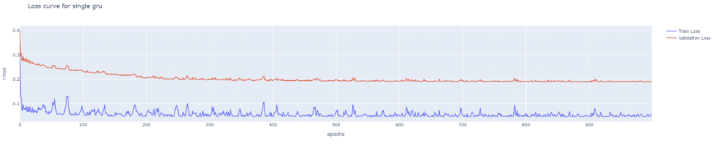
從單層 GRU 的損失曲線可以看出,驗證損失的波動相對較小,並最終穩定於約 0.1 的位置,顯示出模型在驗證集上的穩定性有一定的優勢。然而,訓練損失的波動相對較大,特別是在初期,可能反映出模型對訓練數據特徵的擬合存在一定的問題。
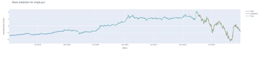
後續再將股價預測圖繪製檢驗模型的預測能力,同樣可發現其預測能力也是較佳的,繪圖程式碼請見最下方。
如同LSTM, 我們也堆疊了一個雙層GRU模型檢驗是否能達成更佳的預測效果。模型架構: 一層GRU + 一層Dropout + 一層GRU+ 一層Dropout + 一層全連接層。其中兩次Dropout的比率都調整為40%,這裡將比率調高的原因是為了避免過擬合問題。
# 建立雙層GRU函式
class GRU(nn.Module):
    def __init__(self):
        super().__init__()
        self.gru1 = nn.GRU(input_size = 4, hidden_size=64, num_layers=1, batch_first=True)
        self.dropout1 = nn.Dropout(0.4)
        self.gru2 = nn.GRU(input_size = 64, hidden_size=32, num_layers=1, batch_first=True)
        self.dropout2 = nn.Dropout(0.4)
        self.linear = nn.Linear(32, 1)
    def forward(self, x):
        x, _ = self.gru1(x)
        x = self.dropout1(x)
        x, _ = self.gru2(x)
        x = self.dropout2(x)
        x = x[:, -1, :]
        x = self.linear(x)
        return x
def trainer(epochs, loader, X_train, y_train, X_val, y_val, model, criterion, optimizer):
    train_loss, test_loss = [], []
    best_rmse = float('inf')
    best_y_true, best_y_pred = None, None
    best_model_state = None
    best_epoch = -1  # 記錄最佳 Epoch

    for epoch in range(epochs):
        model.train()
        for batch, (x, y_true) in enumerate(loader):
            y_pred = model(x)
            loss = criterion(y_pred, y_true)
            loss.backward()
            optimizer.step()
            optimizer.zero_grad()

        model.eval()
        with torch.no_grad():
            y_pred_val = model(X_train)
            train_rmse = np.sqrt(criterion(y_pred_val, y_train).item())
            train_loss.append(train_rmse)
            y_pred_val = model(X_val)
            test_rmse = np.sqrt(criterion(y_pred_val, y_val).item())
            test_loss.append(test_rmse)

            # 儲存最佳結果
            if test_rmse < best_rmse:
                best_rmse = test_rmse
                best_y_true = y_val.cpu().numpy()
                best_y_pred = y_pred_val.cpu().numpy()
                best_model_state = model.state_dict()
                best_epoch = epoch + 1  # 記錄最佳 Epoch

    # 載入最佳模型權重
    model.load_state_dict(best_model_state)
    return train_loss, test_loss, best_y_true, best_y_pred, best_epoch

# 設置模型、損失函數與優化器
model = S_GRU().to(device)
criterion = nn.MSELoss()
optimizer = optim.Adam(model.parameters())
epochs = 1000
# 開始訓練並且計算訓練所需時間
start = time.time()
gru_train_loss, gru_test_loss, gru_y_true, gru_y_pred, gru_best_epoch = trainer(epochs, loader, X_train, y_train, X_val, y_val, model, criterion, optimizer)
print('single gru time cost %.4f' %(end-start))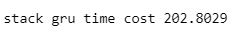
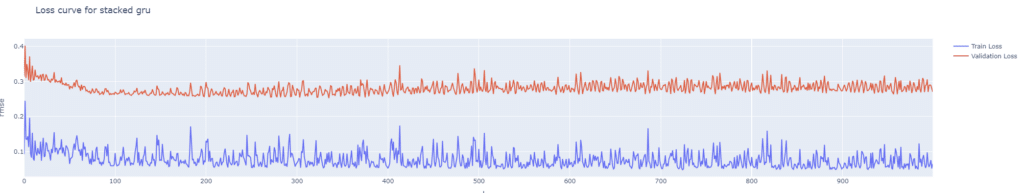
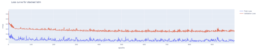
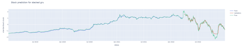
從雙層 GRU 的損失曲線可以觀察到,驗證集的損失最終收斂至約 0.2 的位置。並且其損失曲線的波動幅度明顯比其他三個模型(單層 GRU、單層 LSTM 和雙層 LSTM)都大。這顯示模型的穩定性相對不足。。後續再將股價預測圖繪製檢驗模型的預測能力,同樣可發現其預測能力較單層遜色,繪圖程式碼請見最下方。
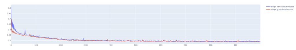
從上述結果可以發現,不論是LSTM或是GRU,單層在台積電股價預測上表現皆優於雙層。接著我們比較兩單層模型在驗證集的損失曲線,可以發現兩者最後都能收斂到0.2附近。在震盪部分事實上兩者幅度相當,但GRU在前期的損失下降幅度明顯大於LSTM,繪圖程式碼見最下方。
值得注意的是,單層 GRU 的訓練時間雖然略慢於單層 LSTM(約慢 29 秒),但雙層 GRU 的訓練時間則顯著超過雙層 LSTM(多出約 104 秒)。這可能是因為 GRU 的結構在單層模型中較為輕量化,但當層數增加時,參數數量的增長對計算資源的需求更加明顯,從而導致運算時間的顯著增加。
綜合來看,如果對運算效率要求較高,單層 LSTM 在速度和性能上可能是一個更為均衡的選擇
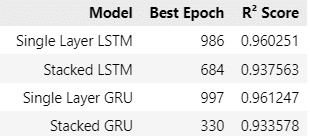
根據表格數據,單層 GRU 在所有模型中表現最佳,達到了最高的 R² Score(0.961247),但需要較多的 Epoch(997)才能達到最佳效果,而單層 LSTM 的 R² Score(0.960251)接近 GRU,且略微需要更少的 Epoch(986)。相較之下,雙層模型(Stacked LSTM 和 Stacked GRU)的 R² Score 較低(分別為 0.937563 和 0.933578),顯示增加模型層數可能導致過擬合或學習效率下降。特別是雙層 GRU,雖然最佳 Epoch 僅為 330,但準確度最低,表明其在此場景下不具優勢。因此,單層模型(特別是單層 GRU)在準確度和學習能力上更具吸引力,適合追求高準確度的應用。
總的說,LSTM與GRU在這次的試驗中,對台積電股價皆有一定的預測能力。由於這次試驗僅採取單一股票標的且時間限縮於2019到2022三年,故無法說明LSTM或GRU對於股價一定具有預測能力。但根據【資料科學】LSTM的結論與本次的觀察,我們認為LSTM與GRU可以作為投資人在選股時的一項參考依據,建議可以搭配其他選股指標,比如: 【實戰應用】布林通道交易策略 或 【量化分析】MACD指標回測實戰,建構投資策略。
溫馨提醒,本次策略與標的僅供參考,不代表任何商品或投資上的建議。之後也會介紹使用TEJ資料庫來建構各式指標,並回測指標績效,所以歡迎對各種交易回測有興趣的讀者,選購TEJ E-Shop的相關方案,用高品質的資料庫,建構出適合自己的交易策略。