
Table of Contents
布林通道(Bollinger Band)是由 John Bollinger 在1980 年代所發明的技術指標。布林通道是由均線和統計學的標準差概念結合而成,均線 (Moving Average),簡稱 MA,代表過去一段時間的平均成交價格,一般來說在布林中使用的時間區段為近20日;標準差 (Standard Deviation),簡稱SD,常以 σ 作為代號,用於表示資料中數值的分散程度。
布林通道總共包含三條線:
由於在長時間觀測下,標的價格的變化會呈現常態分佈 (Normal Distribution),而根據統計學原理,在常態分佈下有 95% 的機率,資料會分布在平均值正負兩倍標準差 (μ − 2σ, μ + 2σ) 之間,也稱為 95% 的信賴區間,而布林通道正是以上述的統計學原理作為理論依據,發展出來的技術指標。
實際交易策略如下:
本文使用 Windows 11 並以 jupyter notebook 作為編輯器。
資料期間從 2021–04–01 至 2022–12–31,以友達光電 (2409) 作為實例。
import pandas as pd
import numpy as np
import tejapi
import os
import matplotlib.pyplot as plt

os.environ['TEJAPI_BASE'] = 'https://api.tej.com.tw'
os.environ['TEJAPI_KEY'] = 'Your Key'
os.environ['mdate'] = '20210401 20221231'
os.environ['ticker'] = '2409'

# 使用 ingest 將股價資料導入暫存,並且命名該股票組合 (bundle) 為 tquant
!zipline ingest -b tquant

from zipline.api import set_slippage, set_commission, set_benchmark, attach_pipeline, order, order_target, symbol, pipeline_output, record
from zipline.finance import commission, slippage
from zipline.data import bundles
from zipline import run_algorithm
from zipline.pipeline import Pipeline
from zipline.pipeline.filters import StaticAssets
from zipline.pipeline.factors import BollingerBands
from zipline.pipeline.data import EquityPricing
Pipeline() 提供使用者快速處理多檔標的的量化指標與價量資料的功能,於本次案例我們用以處理:
def make_pipeline():

    perf = BollingerBands(inputs=[EquityPricing.close], window_length=20, k=2)
    upper,middle,lower = perf.upper,perf.middle, perf.lower
    curr_price = EquityPricing.close.latest

    return Pipeline(
        columns = {
            'upper':  upper,
            'middle':  middle,
            'lower':  lower,
            'curr_price':curr_price
        }
)inintialize 函式用於定義交易開始前的每日交易環境,與此例中我們設置:
def initialize(context):
    context.last_buy_price = 0
    set_slippage(slippage.VolumeShareSlippage())
    set_commission(commission.PerShare(cost=0.00285))
    set_benchmark(symbol('2409'))
    attach_pipeline(make_pipeline(), 'mystrategy')
context.last_signal_price = 0handle_data 函式用於處理每天的交易策略或行動。
def handle_data(context, data):
    out_dir = pipeline_output('mystrategy') # 取得每天 pipeline 的布林通道上中下軌
    for i in out_dir.index:
        upper = out_dir.loc[i, 'upper']
        middle = out_dir.loc[i, 'middle']
        lower = out_dir.loc[i, 'lower']
        curr_price = out_dir.loc[i, 'curr_price']
        cash_position = context.portfolio.cash
        stock_position = context.portfolio.positions[i].amount

        buy, sell = False, False
        record(price = curr_price, upper = upper, lower = lower, buy = buy, sell = sell)

        if stock_position == 0:
            if (curr_price <= lower) and (cash_position >= curr_price * 1000):
                order(i, 1000)
                context.last_signal_price = curr_price
                buy = True
                record(buy = buy)
        elif stock_position > 0:
            if (curr_price <= lower) and (curr_price <= context.last_signal_price) and (cash_position >= curr_price * 1000):
                order(i, 1000)
                context.last_signal_price = curr_price
                buy = True
                record(buy = buy)
            elif (curr_price >= upper):
                order_target(i, 0)
                context.last_signal_price = 0
                sell = True
                record(sell = sell)
            else:
                pass
        else:
pass於本案例使用 matplotlib 將視覺化買賣點與投組價值變化。
def analyze(context, perf):
    fig = plt.figure()
    ax1 = fig.add_subplot(211)
    perf.portfolio_value.plot(ax=ax1)
    ax1.set_ylabel("Portfolio value (NTD)")
    ax2 = fig.add_subplot(212)
    ax2.set_ylabel("Price (NTD)")
    perf.price.plot(ax=ax2)
    perf.upper.plot(ax=ax2)
    perf.lower.plot(ax=ax2)
    ax2.plot( # 繪製買入訊號
        perf.index[perf.buy],
        perf.loc[perf.buy, 'price'],
        '^',
        markersize=5,
        color='red'
    )
    ax2.plot( # 繪製賣出訊號
        perf.index[perf.sell],
        perf.loc[perf.sell, 'price'],
        'v',
        markersize=5,
        color='green'
    )
    plt.legend(loc=0)
    plt.gcf().set_size_inches(18,8)
    plt.show()
使用 run_algorithm 執行上述所編撰的交易策略,設置交易期間為 2021-06-01 到 2022-12-31,所使用資料集為 tquant,初始資金為 500,000 元。其中輸出的 results 就是每日績效與交易的明細表,並且輸出買買點。
觀察以下圖表,可以發現在 2021 年 11 月到 2021 年 12 月的上升區段,由於收盤價無法碰觸到布林通道下界,因此一直沒有買入持有,導致無法賺取這區段的價差。
同樣的問題也出現在連續下降波段,比如 2022 年 4 月開始的下降趨勢,不斷地碰觸布林通道下界,在回漲一小段後,因布林通道上界過低容易碰觸到,所以很快就賣出掉,導致這段期間的交易為負報酬。
事實上,由於20日布林通道的遲滯性,故無法反映短期高波動的價格變化,若您所分析的股票為漲跌幅度較大者,建議縮短布林通道的期間或搭配其他觀察趨勢的指標建立交易策略。
results = run_algorithm(
    start = pd.Timestamp('2021-06-01', tz='UTC'),
    end = pd.Timestamp('2022-12-31', tz ='UTC'),
    initialize=initialize,
    bundle='tquant',
    analyze=analyze,
    capital_base=5e5,
    handle_data = handle_data
)

results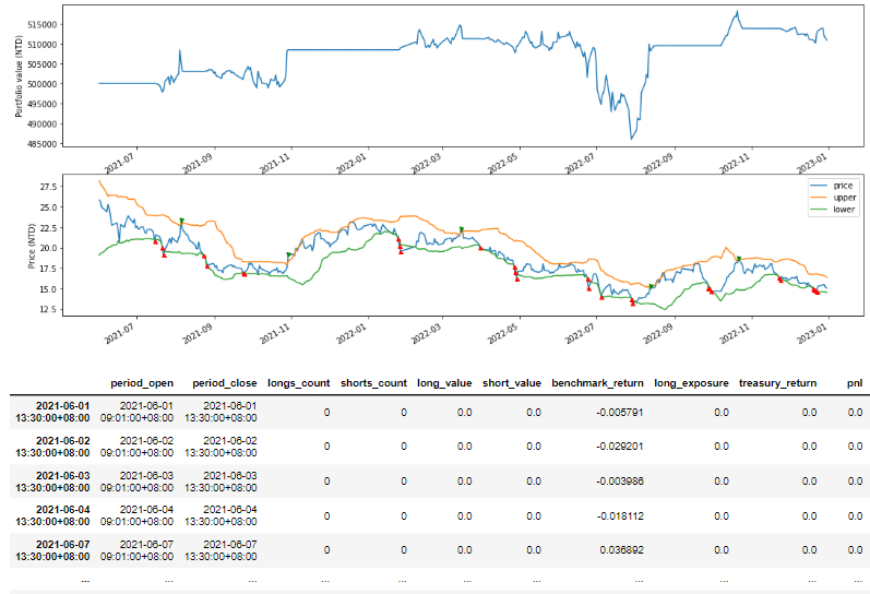
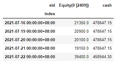
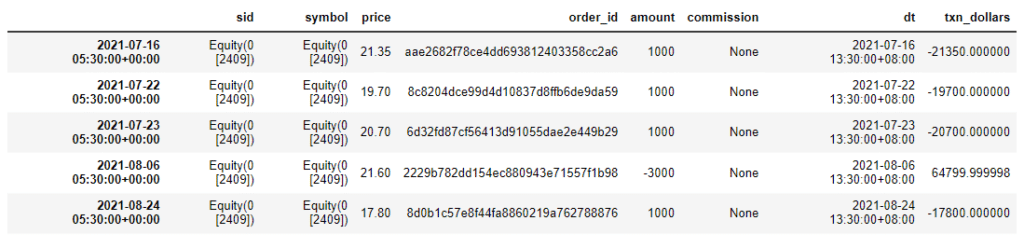
緊接著我們使用 TQuant Lab 隨附的 Pyfolio 模組進行投組的績效與風險分析,首先我們使用 extract_rets_pos_txn_from_zipline() 計算報酬、部位與交易紀錄。
import pyfolio as pf
returns, positions, transactions = pf.utils.extract_rets_pos_txn_from_zipline(results)紀錄每天的投組報酬率。
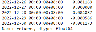
benchmark_rets = results['benchmark_return']
pf.plotting.plot_rolling_returns(returns, factor_returns=benchmark_rets)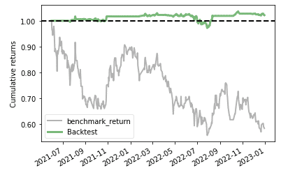
透過 pyfolio 的 show_perf_stats 函式,輕鬆建立策略的績效與風險分析表。
pf.plotting.show_perf_stats(
        returns,
        benchmark_rets,
        positions=positions,
        transactions=transactions)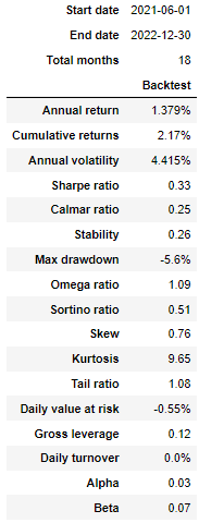
2021後半年到2022整年,對於友達來說是整體緩步向下的趨勢。若採用買進持有的策略,到期日所累績報酬為嚴重的 -40% 到 -50% 之間,相對的,採用布林通道交易策略之下,其表現是優於買進持有的。
然而單純的布林通道策略,在下滑大趨勢區段中後的回升段中,容易有過早出場的劣勢,在上升區段中,容易有極少入場的窘境;故針對股價大幅變動的個股,建議多採用其他判斷趨勢強弱的指標,加以優化自身的策略。
溫馨提醒,本次策略與標的僅供參考,不代表任何商品或投資上的建議。之後也會介紹使用TEJ資料庫來建構各式指標,並回測指標績效,所以歡迎對各種交易回測有興趣的讀者,選購 TEJ E-Shop 的相關方案,用高品質的資料庫,建構出適合自己的交易策略。