
Table of Contents
The origins of the momentum anomaly have long been debated, with multiple competing explanations. Among them, one of the most influential behavioral interpretations attributes momentum to the Disposition Effect, a systematic bias in investor decision-making. This article focuses on the Capital Gain Overhang (CGO) factor, specifically designed to quantify this behavioral bias. Using the Taiwan equity market as a case study, we examine CGO’s predictive power as a stock selection indicator and evaluate its practical value through empirical analysis.
A cornerstone of behavioral finance is Prospect Theory, proposed by Kahneman and Tversky (1979). The theory suggests that individuals evaluate gains and losses relative to a reference point rather than absolute wealth levels, and they experience losses more intensely than equivalent gains—a phenomenon known as loss aversion.
Building on this foundation, Shefrin and Statman (1985) introduced the concept of the Disposition Effect. Within the framework of mental accounting, investors tend to assign each stock purchase to a separate mental account, with the purchase price serving as the critical reference point for gains or losses. This bias drives two systematic behaviors: investors are prone to selling winning stocks too early to lock in gains, while holding onto losing stocks for too long to avoid realizing losses.
If such behavior is widespread, it inevitably creates predictable price pressure. To capture this effect, Grinblatt and Han (2005) proposed the Capital Gain Overhang (CGO) factor, designed to directly quantify the Disposition Effect. CGO measures the gap between the current market price and the estimated average cost basis of all shareholders. Since actual investor costs are unobservable, they introduced a turnover-based method, which approximates cost using a volume-weighted series of historical prices. Subsequent research validated this approach: Frazzini (2006) employed a completely different holding-based method using mutual fund holdings data and reached conclusions highly consistent with Grinblatt and Han. The convergence of these independent methodologies strongly indicates that the CGO effect is genuine, rather than an artifact of any specific estimation technique.
The theoretical implication is straightforward:
This asymmetric reaction creates a positive relationship between CGO and expected future returns.
Most importantly, CGO reinterprets the traditional momentum factor. Grinblatt and Han (2005) demonstrated that CGO not only predicts future returns but also subsumes the explanatory power of the conventional intermediate-term momentum factor. This suggests that the well-documented momentum anomaly may largely be a manifestation of the Disposition Effect. In other words, traditional momentum factors, based purely on past returns, may simply act as a noisy proxy for CGO.

This section presents the empirical examination of the Capital Gain Overhang (CGO) factor in Taiwan’s equity market, focusing on whether it reliably predicts future returns.
The dataset is sourced from Taiwan Economic Journal (TEJ) :
CGO is calculated following Grinblatt and Han’s (2005) turnover-based method, adapted to Taiwan’s market structure. Specifically, TEJ applies a 100-trading-day look-back window, using turnover-weighted adjusted daily prices with time decay to estimate investors’ average cost basis.
This design reflects two key assumptions:
To examine the cross-sectional features of Capital Gain Overhang (CGO) in Taiwan’s stock market, we apply the portfolio-sorting method. On each trading day, all stocks are ranked by their CGO values and divided into ten equally weighted portfolios, labeled from P1 (lowest CGO) to P10 (highest CGO).
Table 1 summarizes descriptive statistics of these portfolios over the sample period (January 2005 – June 2025). The results show that average CGO values increase monotonically from P1 to P10, confirming the effectiveness of the grouping.
Table 1:descriptive statistics of CGO factor
| Min | Max | Mean | Std | Count | % | |
|---|---|---|---|---|---|---|
| 1 | -0.9236 | 0.09118 | -0.194762 | 0.107928 | 735360 | 10.031237 |
| 2 | -0.53369 | 0.12821 | -0.114891 | 0.076839 | 732881 | 9.99742 |
| 3 | -0.46608 | 0.15705 | -0.081821 | 0.07067 | 732350 | 9.990177 |
| 4 | -0.42359 | 0.18262 | -0.057136 | 0.065729 | 732840 | 9.996861 |
| 5 | -0.38765 | 0.20536 | -0.036038 | 0.061512 | 733393 | 10.004405 |
| 6 | -0.34851 | 0.23364 | -0.016373 | 0.057915 | 731802 | 9.982702 |
| 7 | -0.31608 | 0.27171 | 0.003678 | 0.055108 | 732338 | 9.990013 |
| 8 | -0.27466 | 0.3223 | 0.026796 | 0.053688 | 732727 | 9.99532 |
| 9 | -0.22777 | 0.40388 | 0.05915 | 0.055491 | 732306 | 9.989577 |
| 10 | -0.16402 | 3.2241 | 0.151017 | 0.110712 | 734704 | 10.022288 |
An important observation is that the extreme portfolios—P1 (largest unrealized losers) and P10 (largest unrealized winners)—exhibit significantly higher standard deviations than the middle groups. This indicates greater heterogeneity among firms at both ends of the CGO distribution.
We next evaluate the predictive power of CGO for future returns by analyzing the performance of these sorted portfolios.
Table 2 and Figure 3 present the average daily returns of CGO decile portfolios across different holding horizons (1 to 100 trading days). Two key findings emerge:
Table 2:Average Daily Returns of CGO Factor Groups and Long-Short Hedge Portfolios
| 1D | 5D | 10D | 20D | 40D | 60D | 100D | |
|---|---|---|---|---|---|---|---|
| Top Quantile, P10 | 9.964 | 10.178 | 10.275 | 8.820 | 8.293 | 8.226 | 8.026 |
| Bottom Quantile, P1 | 7.626 | 7.322 | 6.486 | 6.465 | 5.387 | 4.279 | 4.046 |
| Spread, P10-P1 | 2.338 | 3.386 | 4.400 | 3.010 | 3.552 | 4.543 | 4.541 |
Figure 3:Average returns of CGO factor deciles over different holding periods
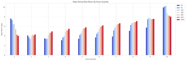
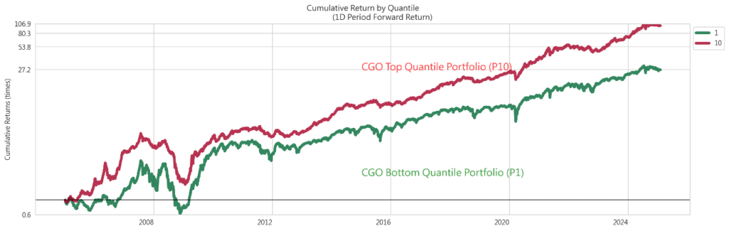
Figure 4 further illustrates cumulative performance. The high-CGO portfolio shows steadily superior cumulative returns compared to the low-CGO portfolio, with smaller drawdowns, suggesting that high-CGO firms may possess a degree of defensiveness in adverse markets. This feature enhances the factor’s ability to generate favorable risk-adjusted returns over the long run.
Figure 4 : Cumulative Return Trends by CGO Group (Top vs. Bottom Quantile)
To test whether the returns of CGO-sorted portfolios can be explained by well-known systematic risk factors, we conduct time-series regressions of monthly excess returns against several classical asset pricing models. At the beginning of each month, stocks are grouped by their end-of-month CGO values, and portfolio returns are held for one month. These returns are then regressed on the factors of four benchmark models. The primary focus of this analysis is the intercept term (alpha). A significantly positive alpha indicates the presence of abnormal returns unexplained by the included risk factors. To account for serial correlation and heteroskedasticity in financial time series, all t-statistics are adjusted using the Newey–West (1987) method.
Table 5:CGO Portfolio Factor Model Regression Alpha
| Portfolio | CAPM | Fama-French 3 Factors | Fama-French 5 Factors | Fama-French 6 Factors |
|---|---|---|---|---|
| Bottom Quantile P1 | 0.0017 (0.58) | -0.0015 (-0.76) | 0.0001 (0.03) | 0.0034 (1.62) |
| Top Quantile P10 | 0.0106*** (5.49) | 0.0082*** (5.69) | 0.0090*** (5.85) | 0.0077*** (5.26) |
| Spread P10-P1 | 0.0088*** (2.81) | 0.0097*** (3.19) | 0.0090*** (2.70) | 0.0043 (1.38) |
Table 5 reports the regression alphas for the lowest-CGO portfolio (P1), the highest-CGO portfolio (P10), and the long–short spread (P10–P1).Key findings are as follows:
To further evaluate the predictive power of CGO, we calculate the Information Coefficient (IC)—the Spearman rank correlation between CGO values and subsequent returns across different holding horizons.
Table 6:Summary of Information Coefficients (ICs) for the CGO Factor at Different Holding Periods
| 1D | 5D | 10D | 20D | 40D | 60D | 100D | |
|---|---|---|---|---|---|---|---|
| IC Mean | -0.001 | 0.0008 | 0.0065 | 0.0079 | 0.0252 | 0.0448 | 0.0635 |
| IC Std | 0.1226 | 0.1369 | 0.1389 | 0.1436 | 0.1415 | 0.1318 | 0.1144 |
| Risk Adjusted IC | -0.008 | 0.0062 | 0.0465 | 0.0552 | 0.1781 | 0.3401 | 0.5554 |
| IC t-value | -0.5649 | 0.4359 | 3.2661 | 3.8777 | 12.5163 | 23.9026 | 39.0314 |
| IC p-value | 0.5721 | 0.663 | 0.0011*** | 0.0001*** | 0*** | 0*** | 0*** |
| IC Skewness | -0.1767 | -0.3965 | -0.4118 | -0.5668 | -0.9367 | -1.1376 | -1.1015 |
| IC Kurtosis | 1.6359 | 1.3835 | 1.1328 | 0.7843 | 1.4874 | 2.3776 | 2.7987 |
Table 6 reports the IC statistics. The results highlight two key insights:
In sum, the IC analysis provides robust evidence that CGO is a powerful predictive signal in Taiwan’s equity market, particularly over 60–100 day horizons, where its forecasting ability is both stable and economically meaningful.
The empirical analysis confirms that Capital Gain Overhang (CGO) is a meaningful and robust factor in Taiwan’s equity market. Across portfolio-sorting tests, return analysis, risk factor regressions, and IC evaluation, CGO consistently shows predictive power, particularly over medium- to long-term horizons. High-CGO portfolios deliver significantly higher future returns, with evidence of positive alpha beyond standard Fama–French factors. However, its overlap with momentum suggests that CGO captures behavioral effects closely tied to the Disposition Effect.
Overall, these findings establish CGO as a reliable behavioral factor with clear economic intuition and strong statistical support. The next step is to translate these insights into Factor Strategy – CGO, where we design and backtest strategies to evaluate how CGO can enhance portfolio performance.」
👉 Continue reading to explore how CGO can be transformed from a predictive factor into actionable investment strategies.