
Table of Contents
First of all, we would implement the process to construct models so as to make you understand the application of python packages. However, in case of redundancy of this article, there is no hypothesis test. Subsequently, we would calculate the forecasted return and price. Last but not least, apply visualization to compare the prediction and actual trend to assess the result of ARMA-GARCH.
Note: we apply “ARMA” in this article, not like the previous one “ARIMA”. The difference is that ARIMA is capable of differencing and dealing with non-stationary data. We conducted ARIMA in previous one to make you understand Time Series profoundly. Here, the use of ARMA would make you know the alternative of Time Series Model.
MacOS & Jupyter Notebook
import numpy as npimport pandas as pdimport matplotlib.pyplot as plt%matplotlib inlineimport seaborn as snssns.set()import tejapitejapi.ApiConfig.api_key = 'Your Key'tejapi.ApiConfig.ignoretz = True
Security Transaction Data Table:Listed securities with unadjusted price and index. Code is ‘TWN/APRCD’.
Step 1. Data Selection, oo5o.TW
data = tejapi.get('TWN/APRCD', # 公司交易資料-收盤價coid= '0050', # 台灣50mdate={'gte': '2003-01-01', 'lte':'2021-12-31'},opts={'columns': ['mdate', 'close_d', 'roi']},chinese_column_name=True,paginate=True)data['年月日'] = pd.to_datetime(data['年月日'])data = data.set_index('年月日')data = data.rename(columns = {'收盤價(元)':'收盤價', '報酬率%':'日報酬率(%)'})
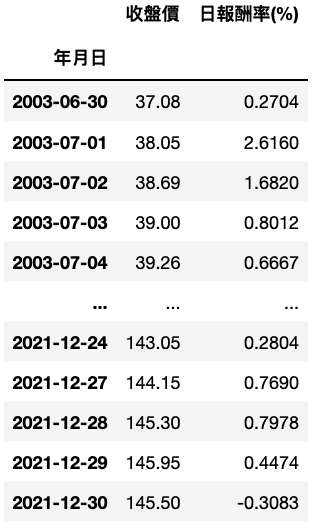
Step 2. Data Split
train_date = data.index.get_level_values('年月日') <= '2020-12-31'train_data = data[train_date].drop(columns = ['收盤價'])test_data = data[~train_date]# 保留test_data收盤價,用來比對模型預測值
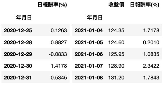
Step 3. Selection of ARMA’s parameters
Here, we apply statsmodels to select parameters, not like the previous article, where we used pmdarima.
import statsmodels.api as sm# AIC、BIC準則sm.tsa.stattools.arma_order_select_ic(train_data, ic=["aic", "bic"])
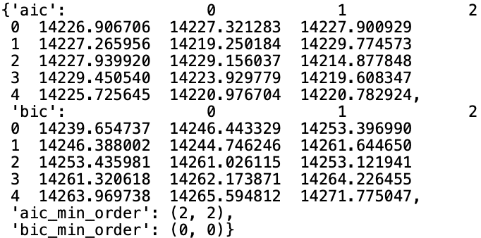
The BIC standard make us apply (p,q) = (0,0), which is derived from that BIC tends to conduct stricter selection on case of multi-variables. Therefore, like the previous article, we would use AIC, (p,q) = (2,2), to construct ARMA.
Step 4. ARMA Model
from statsmodels.tsa.arima_model import ARMAmodel = ARMA(train_data, order = (2, 2))arma = model.fit()print(arma.summary())
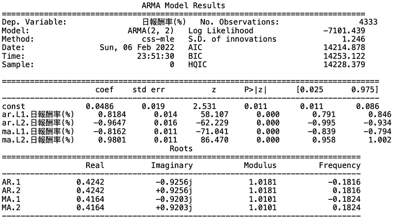
Step 5. GARCH Model
# 取得ARMA模型的殘差項目arma_resid = list(arma.resid)from arch import arch_modelmdl_garch = arch_model(arma_resid, vol = 'GARCH', p = 1, q = 1)garch = mdl_garch.fit()print(garch.summary())
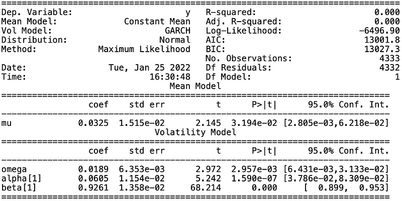
We apply ARMA to forecast the average and GARCH to modify the prediction interval.
Step 1. Average Return Forecasting
# len(train_data) = 4333, len(data) = 4577
forecast_mu = arma.predict(start = 4333, end = 4576)
# 預測函式的end包含當期,所以需進行4577-1=4576。
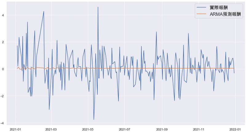
According to above chart, we find that forecasted average return would gradually approach to 0. Fluctuations mainly happens during initial period.
Step 2. Volitility Forecasting
garch_forecast = []for i in range(len(test_data)):train = arma_resid[:-(len(test_data)-i)]model = arch_model(train, vol = 'GARCH', p = 1, q = 1)garch_fit = model.fit()prediction = garch_fit.forecast(horizon=1)garch_forecast.append(np.sqrt(prediction.variance.values[-1:][0]))
Implementing rolling forecasting to predict every single period. Hence, we code in the way making GARCH contained in the loop and store values in the list. Subsequently, we add above forecasted values to “test_data” table and compute upper and lower limits of interval.
test_data['ARMA預測報酬(%)'] = list(forecast_mu)test_data['GARCH預測波動度'] = (garch_forecast)test_data['預測區間上限'] = test_data['ARMA預測報酬(%)'] + test_data['GARCH預測波動度']test_data['預測區間下限'] = test_data['ARMA預測報酬(%)'] - test_data['GARCH預測波動度']
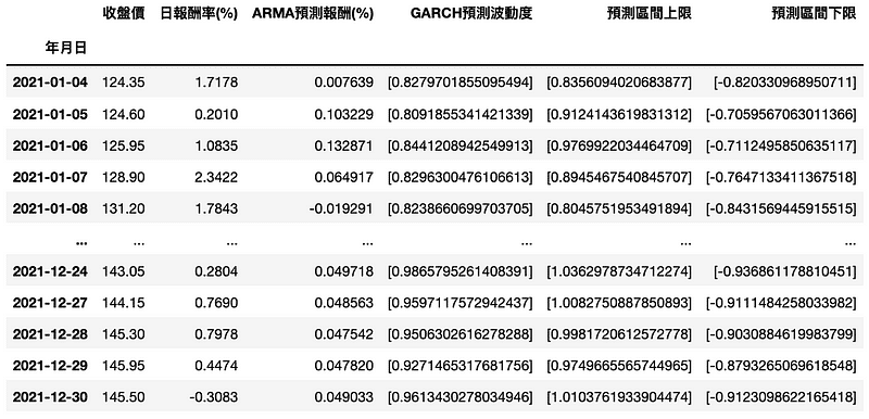
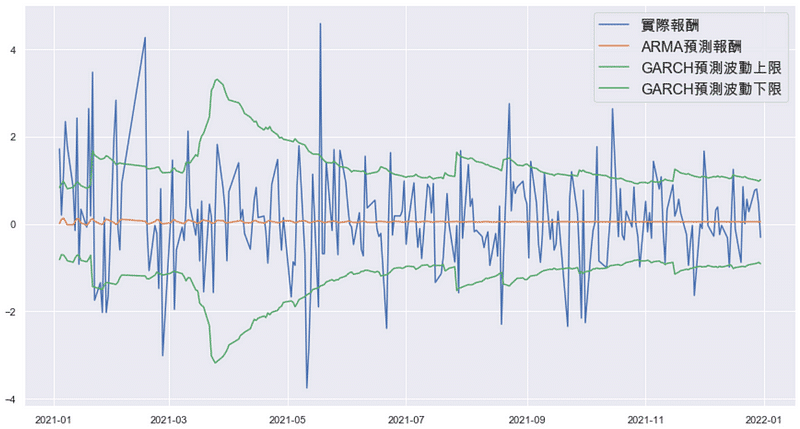
By above chart, it is clear that most of actual returns are in the interval. However, the individual return of much volatility cannot be predicted accurately.
Step 3. Price Forecasting
# 本文已經把train_data中的價格刪除,所以需重新計算2020-12-30的收盤價first_price = test_data['收盤價'][0] / (1+test_data['日報酬率(%)'][0]*0.01)# 計算第一期預測test_data['ARMA預測價格'] = first_price * (1 + test_data['ARMA預測報酬(%)']*0.01)test_data['預測價格區間上限'] = first_price * (1 + test_data['預測區間上限']*0.01)test_data['預測價格區間下限'] = first_price * (1 + test_data['預測區間下限']*0.01)# 計算剩餘預測區間for i in range(1, len(test_data)):test_data['ARMA預測價格'][i] = test_data['預測價格'][i-1] * (1 + test_data['ARMA預測報酬(%)'][i]*0.01)test_data['預測價格區間上限'][i] = test_data['預測價格區間上限'][i-1] * (1 + test_data['預測區間上限'][i]*0.01)test_data['預測價格區間下限'][i] = test_data['預測價格區間下限'][i-1] * (1 + test_data['預測區間下限'][i]*0.01)# 計算區間均價test_data['預測平均價格'] = (test_data['預測價格區間上限'] + test_data['預測價格區間下限']) / 2
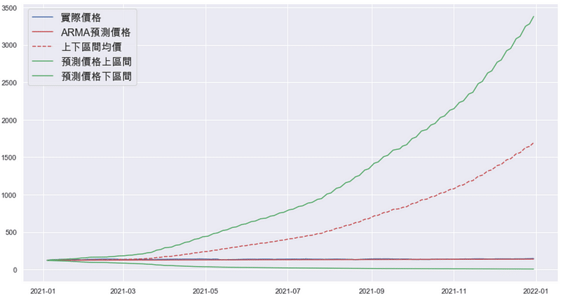
By above chart, we find that the interval expands dramatically with time elapsing. Therefore, it is not reliable enough to assess the result of prediction. we would show the first 2 month and make the conclusion.
new_date = test_data.index.get_level_values('年月日') <= '2021-03-01'new_test = test_data[new_date]
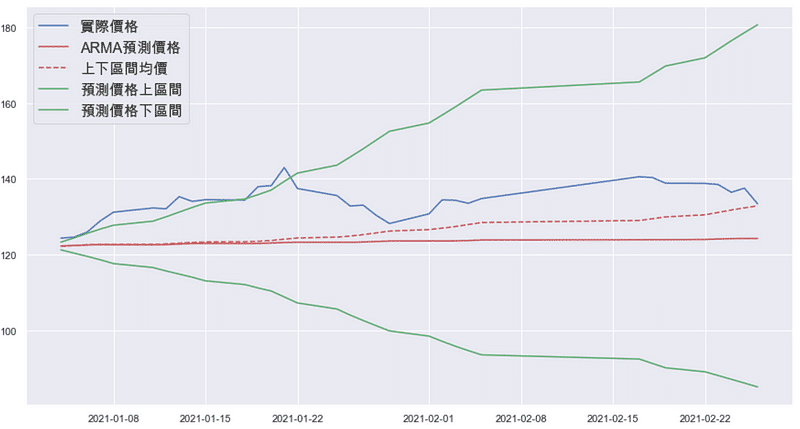
With the period of first two month, it is clear to observe the difference between prediction and actual data. Firstly, the interval average is closer with actual price trend than that of ARMA prediction. As for the interval prediction, we can find that the actual trend does not fall in the interval area until late January.
Based on the last result, you would understand that performance of ARMA-GARCH model on 0050 is not reliable enough, despite the well-fitted model summary. We regard the increasingly wide interval as normal since forecasting should be more conservative with the farther prediction period. Nevertheless, according to first two month chart, we can tell that actual price exceeds predicted interval, which indicates that there is no reliability during the initial period. What brings about the situation may be the lacking consideration about seasonal or exogenous variable. Hence, if you are interested in relative issues, keep reading our articles. To boot, welcom to purchase the plans offered in TEJ E Shop and use the well-complete database to implement your own prediction.