Use free database to do backtesting

Table of Contents
MACD, standing for moving average convergence divergence, can be used to identify the medium-term and long-term trend of stock price. If the fast line (DIF) crosses from below to above the slow line(MACD), indicating there’s an upside momentum. On the contrary, when the fast line crosses from above to below the slow line, the stock price is more likely to go up in the future. Since this kind of indicator can produce clear signals, it’s proper to backtest the performance of strategies based on it.
An effective backtesting should not only have clear signals, but also have to take the timing of the occurrence of signals, transaction fee and the minimum charge of it, and transfer tax into consideration. When calculating the return of the strategy, cash position in hand should also be considered to have a more realistic performance evaluation of participating in the stock market.
Windows OS and Jupyter Notebook
#Basic function
import numpy as np
import pandas as pd#Visualization
import plotly.graph_objects as go
from plotly import subplots#TEJ
import tejapi
tejapi.ApiConfig.api_key = "Your Key"
tejapi.ApiConfig.ignoretz = True
stock_data = tejapi.get('TRAIL/TAPRCD',
            coid= '3481',
            mdate={'gte': '2020-01-01', 'lte': '2020-12-31'},
            opts={'columns': ['coid', 'mdate', 'open_d','close_d']},
            chinese_column_name=True,
            paginate=True)
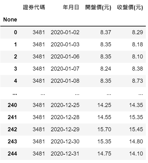
We choose Innolux Corporation (3481) as an example and the columns include opening price, which is used to calculate buying and selling price, and closing price that will produce buy and sell signal.
stock_data['12_ema'] = stock_data['收盤價(元)'].ewm(span = 12).mean()
stock_data['26_ema'] = stock_data['收盤價(元)'].ewm(span = 26).mean()
stock_data['dif'] = stock_data['12_ema']  - stock_data['26_ema']
stock_data['macd'] = stock_data['dif'].ewm(span = 9).mean()
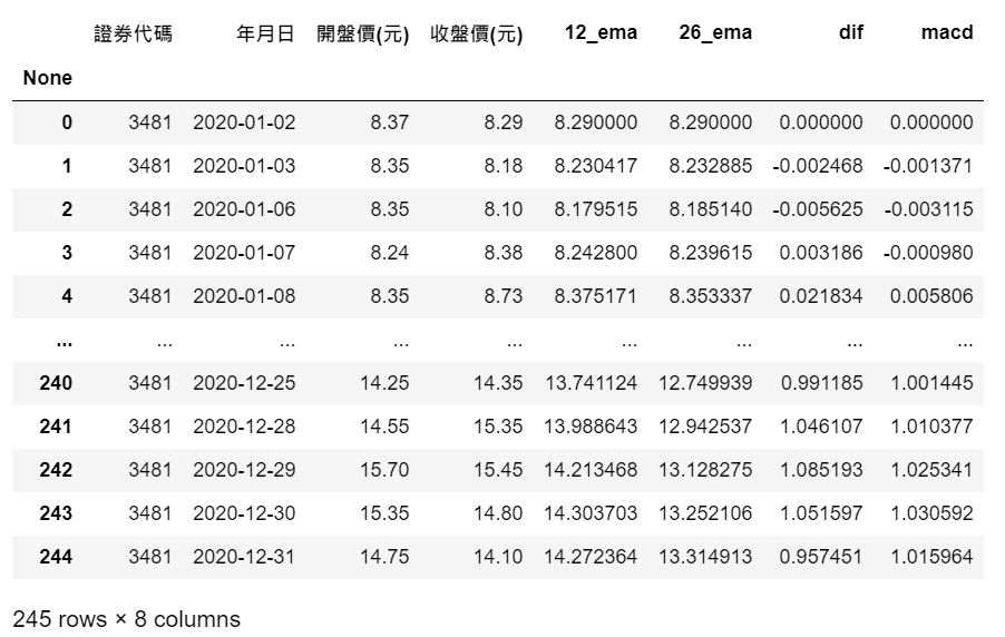
Then we use the closing price to calculate the MACD. First of all, ewm().mean() is applied to produce 12-day and 26-day exponential moving averages. The difference between these two averages is fast line (DIF). If we further take 9-day exponential moving average of fast line, then we get the slow line (MACD)
stock_data['買賣股數'] = 0 #golden cross
stock_data['買賣股數'] = np.where((stock_data['dif'].shift(1)>stock_data['macd'].shift(1)) & (stock_data['dif'].shift(2)<stock_data['macd'].shift(2)), 1000, stock_data['買賣股數'])#death cross
stock_data['買賣股數'] = np.where((stock_data['dif'].shift(1)<stock_data['macd'].shift(1)) & (stock_data['dif'].shift(2)>stock_data['macd'].shift(2)), -1000, stock_data['買賣股數'])
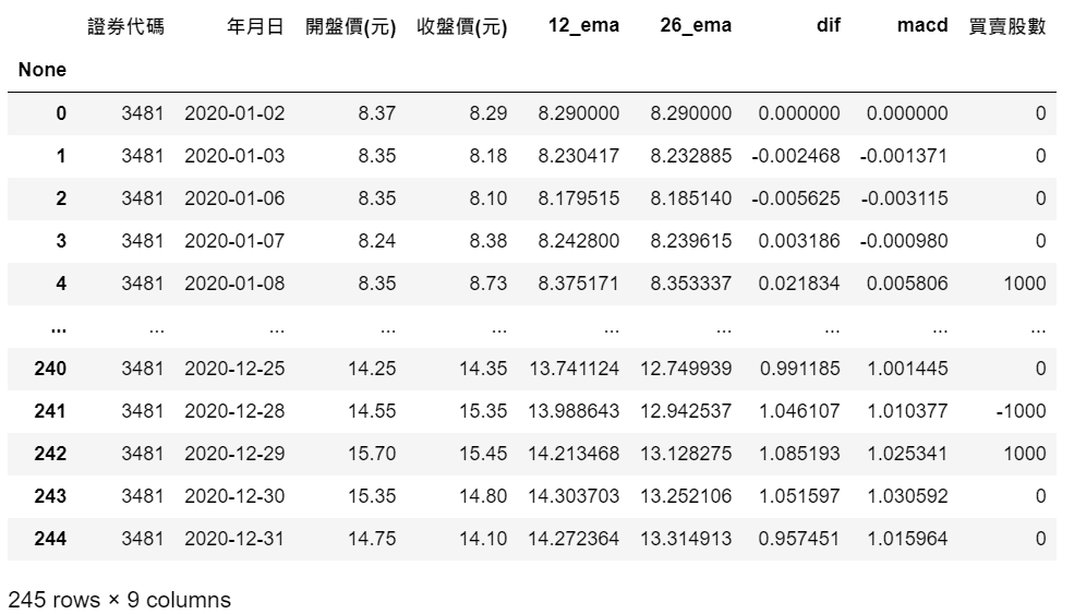
Once the fast line and slow line are calculated, then we can start to build the signals of buying and selling. If the DIF was still lower than the MACD two days ago, but suddenly surpassed the MACD yesterday, meaning there was a ‘golden cross’ yesterday. Since the buying signal popped up after the market closed, we’ll buy 1000 shares at opening price the next day. Similarly, if death cross occurs, we are going to sell 1000 shares at opening price the next day.
stock_data['手續費'] = stock_data['開盤價(元)']* abs(stock_data['買賣股數'])*0.001425
stock_data['手續費'] = np.where((stock_data['手續費']>0)&(stock_data['手續費'] < 20), 20, stock_data['手續費'])
stock_data['證交稅'] = np.where(stock_data['買賣股數']<0, stock_data['開盤價(元)']* abs(stock_data['買賣股數'])*0.003, 0)
stock_data['摩擦成本'] = (stock_data['手續費'] + stock_data['證交稅']).apply(np.floor)
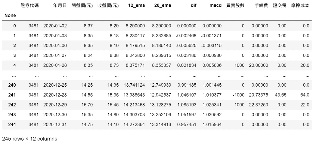
Here comes the friction costs which include transaction fees(0.1425%) and transfer tax (0.3%) in Taiwan. When we buy the stock, the cost incurred is the transaction fee. It’s worth noting here that there’s a minimum charge of 20 NTD for transaction fees if the dealers don’t offer any discount. While we sell the stock, what we need to afford is both transaction fees and transfer fee
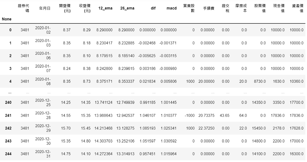
stock_data['股票價值'] = stock_data['買賣股數'].cumsum() * stock_data['收盤價(元)']
stock_data['現金價值'] = 10000 - stock_data['摩擦成本'] + (stock_data['開盤價(元)']* -stock_data['買賣股數']).cumsum()
stock_data['資產價值'] = stock_data['股票價值'] + stock_data['現金價值']
Suppose we have 10,000 NTD at the beginning. Total asset value equals stock position plus cash position. The value of stock position fluctuates with the number of holding shares and stock price; while the value of cash position changes with buying or selling actions, and also the friction costs incurred.
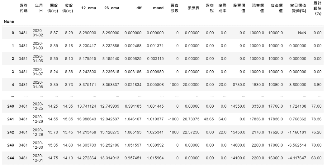
stock_data['當日價值變動(%)'] = (stock_data['資產價值']/stock_data['資產價值'].shift(1) - 1)*100
stock_data['累計報酬(%)'] = (stock_data['資產價值']/10000 - 1)*100
Next we can calculate the daily change in total asset value and cumulative return
Here we can see this strategy does capture some trend and earn the profits. However, it’s risky when stock price barely changes in some periods and keep triggering buying and selling points
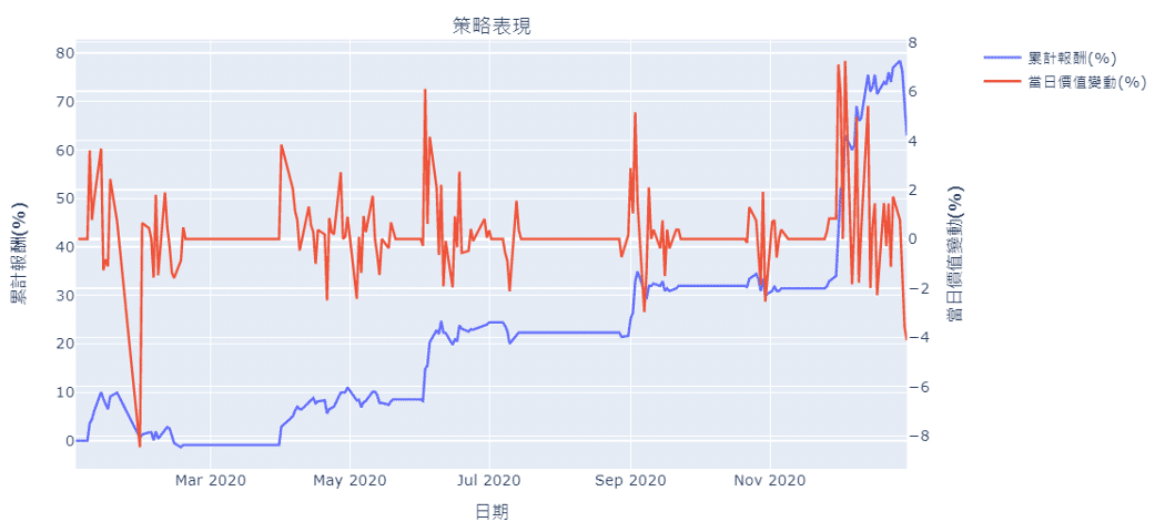
As we can see in the picture, the daily total asset value changes within 8%. If there’s no change, it means the stock price remains the same or we only hold cash. The cumulative return is around 63% at the end, better than the 2020 Taiwan stock market performance.
Readers may find out that this kind of strategy may result in overtrading and incur lots of friction costs, which leads to its performance could be worse than buy and holding strategy. The amount of beginning capital also shows the importance of asset allocation. If we hold too much cash in hand, the overall return will decrease, but the daily volatility could be lower as well. In fact, to get closer to the strategy performance in real life, we should also consider the dividend or other corporate policies that affect stock price. The reason to choose unadjusted stock price in this article is because we want to show the buying and selling points at that time. Furthermore, we may short the stock for some firms with regard to this strategy, then we also have to consider margin issues. But for Innolux Corporation, we have no shorting action. If readers want to backtest longer periods or access more data, welcome to TEJ E-Shop to choose your own optimal plan!
