
Building the financial dashboard through python. ( the top 5 buy list of the foreign & other investors, and combine the trading volume of foreign investors with the stock price.)
Table of Contents
We have introduced some functions of the most-used python packages such as matplotlib, numpy, and pandas in previous articles. In this episode, we will further introduce the application of those packages.
As an investor, it’s your daily routine to spend time watching some statistical data or summary reports of the market after the market is closed. Therefore, each time before you start to observe these data, you will have to go to the TWSE’s website to download the most recent data, then open it on excel to plot and summarize. This kind of work sometimes annoys people because you do the same thing every day. To be honest, it’s totally a waste of time. Compared to execute the same action daily by ourselves, using python seems much more attractive and efficient.
The purpose of this article is to share how we process data, make a plot, and customize your financial dashboard through python🏄🏄~
import tejapi
import pandas as pd
import numpy as np
import matplotlib.pyplot as plt
import datetime
tejapi.ApiConfig.api_key = ‘your key’1️⃣ Get the stock code of the listed company
# 撈取上市所有普通股證券代碼
stk = tejapi.get('TWN/EWNPRCSTD'
                  ,paginate = True
                  ,chinese_column_name = True)code = stk['證券碼'][(stk['證券種類名稱']=='普通股')&(stk['上市別']=='TSE')].to_list()
code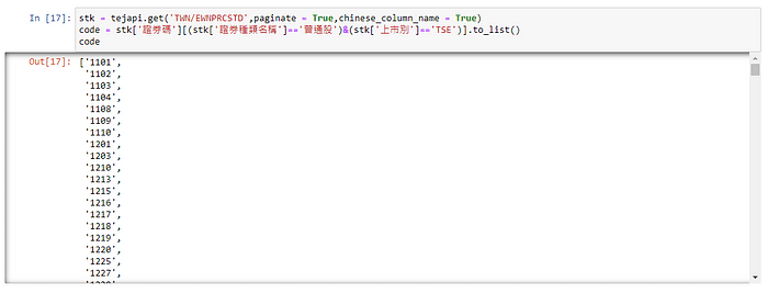
2️⃣ Get foreign & other investors daily trading summary
# 撈取法人買賣超(日)
buyover = tejapi.get('TWN/EWTINST1'
             ,coid=code
             ,mdate = {'gte':'2021-01-01'}
             ,paginate = True
             ,chinese_column_name = True)
# 修改日期格式
buyover['日期'] = buyover['日期'].apply(lambda x: pd.to_datetime(x).date())
buyover['日期'] = buyover['日期'].astype('datetime64')
buyover[buyover['日期']>='2021-03-20']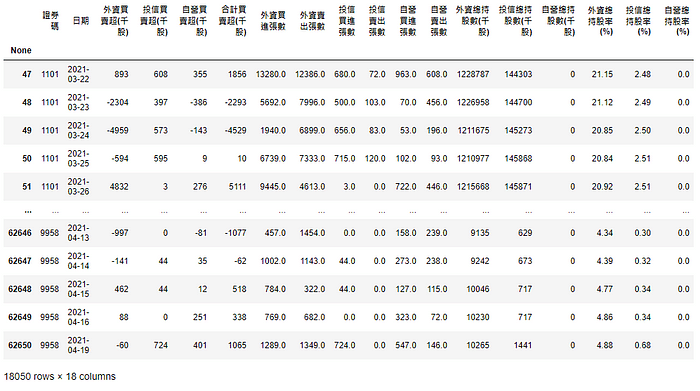
3️⃣ Get stock data
# 撈取股價資料
stock_price =  tejapi.get('TWN/EWPRCD',
                          coid = code,
                          mdate={'gte':'2021-03-20'},
                          opts={'columns':['coid','mdate','open_d', 'high_d','low_d','close_d','volume']}
                          ,paginate = True,chinese_column_name = True)
# 調整日期格式
stock_price['日期'] = stock_price['日期'].apply(lambda x: pd.to_datetime(x).date())
stock_price['日期'] = stock_price['日期'].astype('datetime64')
stock_price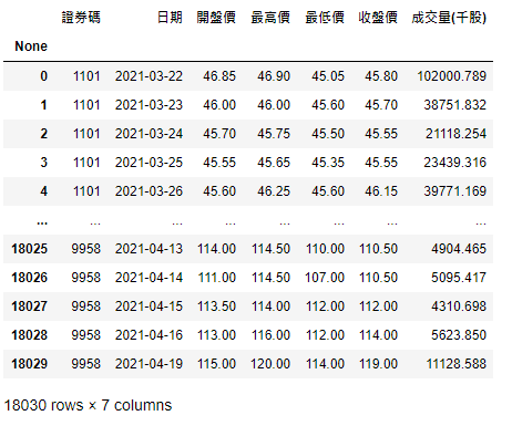
Calculating the monthly trading volume and sorting the trading volume of foreign investors, investment trust, and proprietary respectively.
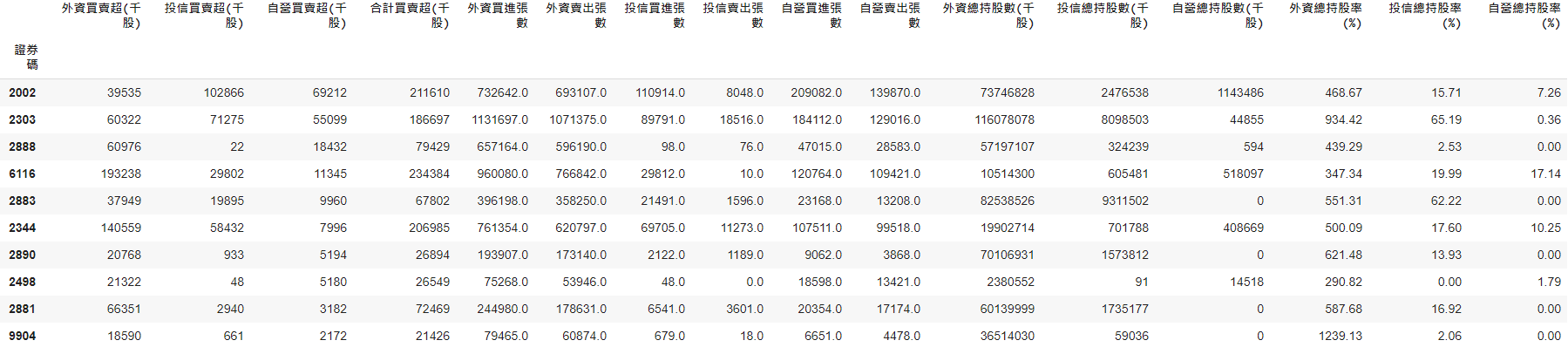
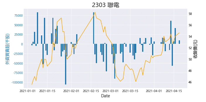
1️⃣ The top 10 buy list in foreign investors are 6116, 2891, 2344, 2352, 2363, 2882, 3711, 2449, 2881, 1303. Most of them are from financial, display, and semiconductor-related industry.
2️⃣ The top 10 buy lists in investment trusts are 3481, 2409, 2002, 2610, 2303, 2603, 2344, 1440, 6116, 2606. The investing style of investment trusts is different from foreign investors. Besides the display and memory industry, the traditional industry(shipping, iron & textile)accounts for the most.
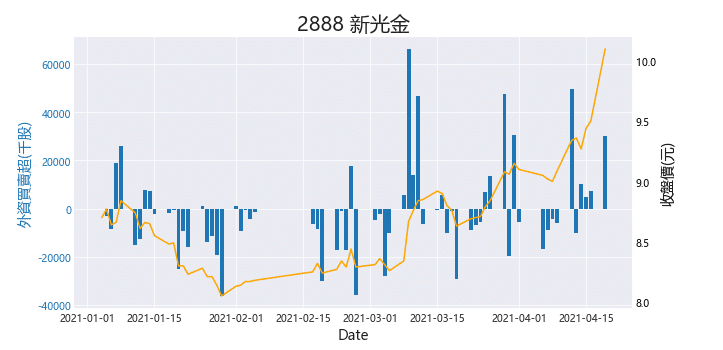
3️⃣ The top 10 buy list in proprietaries are 2002, 2303, 2888, 1314, 2409, 1101, 6116, 3481, 2027, 2883. Their attitude of investing is similar to investment trusts. Their capitals distribute on the display, traditional, and financial industry at the same time.
According to the data, the intersection among the three is the display industry. The domestic investors have the same view based on the trading volumes, and both of them put quite a large percentage of their capital in the traditional industry. However, foreign investors distribute more in the financial and tech sectors.
sorted_fi = buyover[buyover['日期']>'2021-03-20'].groupby(by='證券碼').sum().sort_values(by='外資買賣超(千股)',ascending = False)
sorted_fi[:10]
sorted_it = buyover[buyover['日期']>'2021-03-20'].groupby(by='證券碼').sum().sort_values(by='投信買賣超(千股)',ascending = False)
sorted_it[:10]
sorted_pro = buyover[buyover['日期']>'2021-03-20'].groupby(by='證券碼').sum().sort_values(by='自營買賣超(千股)',ascending = False)
sorted_pro[:10]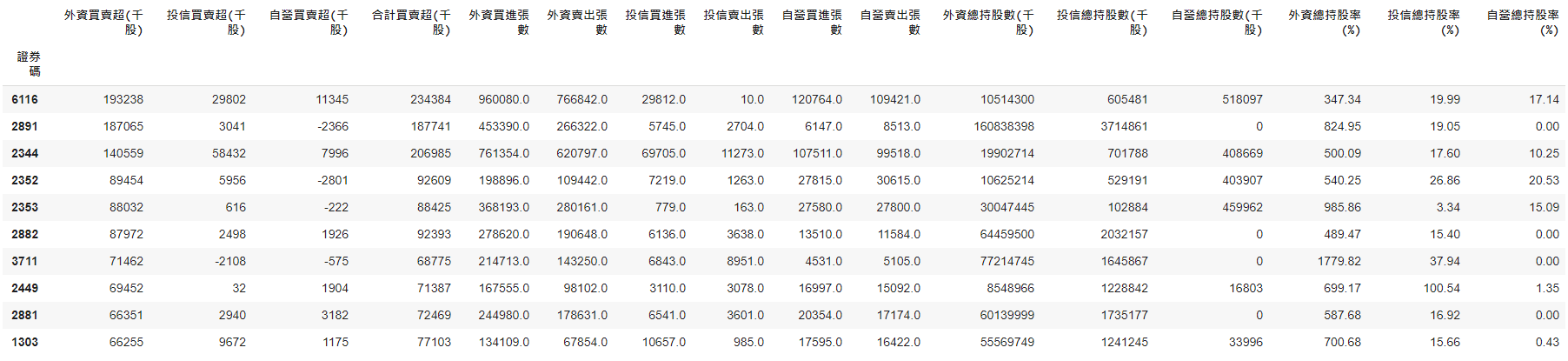
Filter:All of the monthly trading volume of foreign & other investors are positive.
After filtering, we also sort the monthly trading volume of foreign investors, investment trusts, and proprietary respectively.
sorted_fi[(sorted_fi['外資買賣超(千股)']>0)&(sorted_fi['投信買賣超(千股)']>0)&(sorted_fi['自營買賣超(千股)']>0)][:10]
sorted_it[(sorted_it['外資買賣超(千股)']>0)&(sorted_it['投信買賣超(千股)']>0)&(sorted_it['自營買賣超(千股)']>0)][:10]
sorted_pro[(sorted_pro['外資買賣超(千股)']>0)&(sorted_pro['投信買賣超(千股)']>0)&(sorted_pro['自營買賣超(千股)']>0)][:10]

buy_table : The data frame for storing top 5 buy list at different periods.
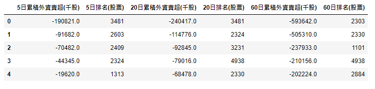
sell_table : The data frame for storing top 5 sell list at different periods.
xx : Calculate the monthly trading volume of the stocks under 5, 20, 60-days.
x.insert() : Insert the column which is named according to its stock code, and the value is xx.
x : The data frame for storing the monthly trading volume of the multi-stocks under the same period.
x.loc[len(x)-1] : Call the most recent data of x.
sort_values(ascending=False)[:5]: Sorting data and choose the top 5
reset_index(drop=True) : Reset the index of data frame.
buy_table = pd.DataFrame()
sell_table = pd.DataFrame()
for i in [5,20,60]:
    x = pd.DataFrame()
    for stock in code:
        # i日累積買賣超
        xx = buyover['外資買賣超(千股)'][buyover['證券碼']==stock].rolling(i).sum().reset_index(drop=True)
        x.insert(loc=0,column=stock,value=xx)
    # 買超排名前5
    buy_table[str(i)+'日累積外資買超(千股)'] = x.loc[len(x)-1].sort_values(ascending=False)[:5].reset_index(drop=True)
    buy_table[str(i)+'日排名(股票)'] = x.loc[len(x)-1].sort_values(ascending=False)[:5].index
    # 買超排名前5
    sell_table[str(i)+'日累積外資賣超(千股)'] = x.loc[len(x)-1].sort_values(ascending=True)[:5].reset_index(drop=True)
    sell_table[str(i)+'日排名(股票)'] = x.loc[len(x)-1].sort_values(ascending=True)[:5].index
buy_table
sell_table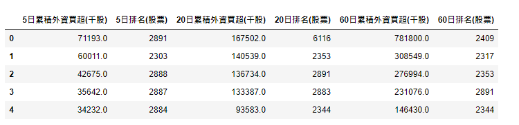
plt.style.use : Set the style of plot.
plt.rcParams[‘font.sans-serif’]=[‘Microsoft YaHei’] : Set the font. There is no Chinese font in the python internals. You need to import additional fonts to display Chinese.
stock = input() : Input the stock code.
FI1.twinx() : Share the x-axis of FI1.
# 調整畫圖模組
plt.style.use('seaborn-darkgrid')
# 調整字體
plt.rcParams['font.sans-serif']=['Microsoft YaHei']
# 可自行輸入股票代號
stock =input()
title = stock+' '+stk['證券名稱'][stk['證券碼']==stock].to_list()[0]
fig, FI1 = plt.subplots(figsize=(10,5))
plt.title(title,{'fontsize' : 20})
plt.xlabel('Date', fontsize=14)
price = FI1.twinx()
# 設定買賣超金額
FI1.set_ylabel('外資買賣超(千股)',color='tab:blue', fontsize=14)
FI1.bar(x=buyover['日期'][buyover['證券碼']==stock]
        ,height=buyover['外資買賣超(千股)'][buyover['證券碼']==stock]
        ,width = 0.8)
FI1.tick_params(axis='y',labelcolor = 'tab:blue')
# 設定收盤價
price.set_ylabel('收盤價(元)'
                 ,color='black'
                 ,fontsize=14)
price.plot(stock_price['日期'][stock_price['證券碼']==stock]
           ,stock_price['收盤價'][stock_price['證券碼']==stock]
           ,color='orange'
           ,alpha=3)
#plt.xticks(rotation=45)
price.tick_params(axis='y',labelcolor = 'black')
# 取消 price的 grid
price.grid(False)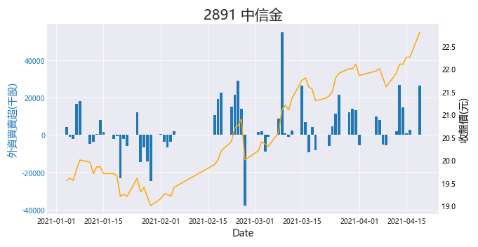
There are hundreds of ways to make charts and plots. We introduced how to implement the charts we often see through python. After all, one of the great benefits of learning python is that it can reduce tedious routines. If you like the topic such as integrating charts, you can leave a message below to tell us. In the future, we will continue to share the application of python in the investment field, please wait and see ❗️❗️
In addition, you can also explore more functions through the official website of these packages~
Finally, if you like this topic, please click 👏 below, giving us more support and encouragement. Additionally, if you have any questions or suggestions, please leave a message or email us, we will try our best to reply to you.👍👍
