Constructing a Custom ESG Investment Portfolio Using the TESG Database

Table of Contents
Article difficulty.:★★☆☆☆
Reading Recommendation: This article is divided into two parts. The first part introduces the percentage of TEJ’s TESG ratings in the components of popular ESG ETFs in the domestic market. The second part will further utilize TESG ratings to construct an investment portfolio with growth potential and sustainable operations. It is recommended that readers start by reading the article Practical Application: ESG Investment Portfolio (Part 1)” to gain a better understanding of this article.
In the previous article, we introduced TESG’s scoring mechanism in detail and its proportion of constituent stocks on domestic popular ETFs. This article will teach readers how to further use the ESG rating provided by TESG, and use Python to construct a An investment portfolio that combines sustainable operations and financial growth. The screening criteria used in this paper are as follows:
The company’s TESG grades for the year were B-, B, B+, A, A+
The CAGR of recurring after-tax net profit in the past year has reached more than 20% (inclusive).
After-tax ROE for the quarter was greater than the industry ROE median for the quarter.
The market value in the current quarter is at least greater than 1 billion yuan.
After screening, use the dividend yield rate in the past three years * 80% + the dividend yield rate in the past year * 20% to calculate the dividend score of the stock, and select the 20 stocks with the highest scores as constituent stocks, and allocate weights based on this score. Rebalancing is carried out on the annual financial report announcement day (end of March, May, August, and mid-November).
*Note: The word index in this article is just a synonym for investment group, please don’t pay attention to it.
Editing environment and module requirements
This article uses Windows OS and uses Jupyter as the editor.
import tejapi as tej
import pandas as pd
import numpy as np
import datetime
import matplotlib.pyplot as plt
import ffn

tej.ApiConfig.api_key = 'Your Key'

plt.rcParams['font.family'] = 'Noto Sans TC'

import warnings
warnings.filterwarnings("ignore")

%matplotlib inline
Securities Attribute Database(TWN/ANPRCSTD)
Listing (cabinet) adjusted stock price (day) – ex-dividend adjustment (TWN/APRCD1)
IFRS focuses on consolidation (single quarter) – All IndustriesⅣ(TWN/AIFINQ)
Download the stock prices of all listed OTC (including unlisted OTC) stocks from January 2010 to November 2022. The fields include adjusted closing price, market value and dividend yield.
#Listed company code
code = tej.get('TWN/ANPRCSTD', mdate={'lt':'2022-11-18'}, chinese_column_name=True, paginate=True)
all_code = code[(code['證券種類名稱'].isin(['普通股', '外國企業來台掛牌', 'TDR'])) & (code['上市別'].isin(['TSE', 'OTC', 'DIST']))]['證券碼'].to_list()  #Those that have been delisted also include

m = pd.date_range('2010-01-01', '2022-11-18', freq='1M', inclusive='both').to_list()

price = pd.DataFrame()

for i in range(1, len(m)):
    price = pd.concat([price, tej.get('TWN/APRCD1',
                                coid=all_code,
                                mdate={'gt': m[i-1], 'lt':m[i]+pd.Timedelta(days=1)},
                                opts={'columns': ['coid', 'mdate', 'close_adj', 'mv', 'div_yid']},
                                chinese_column_name=True,
                                paginate=True)])
    print(f'目前週期:{m[i-1]}:{m[i]}')

price = price.reset_index(drop=True)
price = price.rename(columns={'證券代碼':'公司', '年月日':'年/月'})
price['公司'] = price['公司'].astype(int)
price = price.astype({'年/月':'datetime64[ns]'})
price['y'] = price['年/月'].dt.year
For the ESG level of each company, please go to TEJ PRO → TESG Sustainability Solutions → TESG Sustainability Indicators → TESG Sustainability Indicators Master Table to download the latest version (2021) of information.
tesg = pd.read_csv('TESG_1118.csv')

tesg['證券代碼'] = tesg['證券代碼'].str.extract('(\d+)').astype(int)

tesg['年'] = tesg['年月'].map({201512:2015, 201612:2016, 201712:2017, 201812:2018, 201912:2019, 202012:2020, 202210:2021})

tesg = tesg[['證券代碼', '年', 'TESG等級']]

tesg = tesg[tesg['TESG等級'].isin(['A', 'A+', 'B+', 'B', 'B-'])]

tesg_rank = tesg.pivot(index='證券代碼', columns='年', values='TESG等級').fillna(0)
The financial report data can also be downloaded through TEJ PRO or Python API, select the consolidated-based short form (single quarter)-full industry, and download the financial report of all columns from January 2010 to November 2022.
In addition, it should be noted that, using the time of the financial report release date, the financial report release time of each stock is uniformly set at the end of March, May, August, and mid-November, so as to avoid using incorrect financial report time to screen individual stocks. The last day stipulated.
First, identify the stocks and time that meet the standards in each period, calculate the cumulative return rate of these stocks during this period, and then multiply it by np.dot and the corresponding individual equity weight to obtain the cumulative return rate of each period. , we use 1000 points as the initial value to observe its growth. The earliest batch of stocks are selected from 2015/05/15 and the cumulative returns are calculated.
def cul_index(price, df, init):
    #Convert prices to array type
    price_nd = price.pivot(columns='公司', index='年月', values='收盤價(元)')
    #Fetch all cycles
    period = df['年月'].drop_duplicates().to_list()
    #Remove all companies
    company = [list(df.groupby('年月'))[i][1]['公司'].to_list() for i in range(len(list(df.groupby(['年月']))))]
    #Remove all weight distributions
    weights = [list(df.groupby('年月'))[i][1]['權重分配'].to_list() for i in range(len(list(df.groupby(['年月']))))]

    init = init
    index = []

    for i in range(1, len(weights)):
        index.append((price_nd.loc[period[i-1]: period[i], company[i-1]].pct_change()+1).cumprod().dot(init * np.array(weights[i-1])))
        init = index[-1][-1]
        print(f'第{i}次再平衡:{init:8.2f}')
    index.append((price_nd.loc[period[-1]: pd.Timestamp(2022, 11, 18), company[-1]].pct_change()+1).cumprod().dot(init * np.array(weights[-1]))) #最後一期
    #print(f'第{i+1}次再平衡:{init:8.2f}')

    return pd.DataFrame(pd.concat(index).dropna(), columns=['指數'])
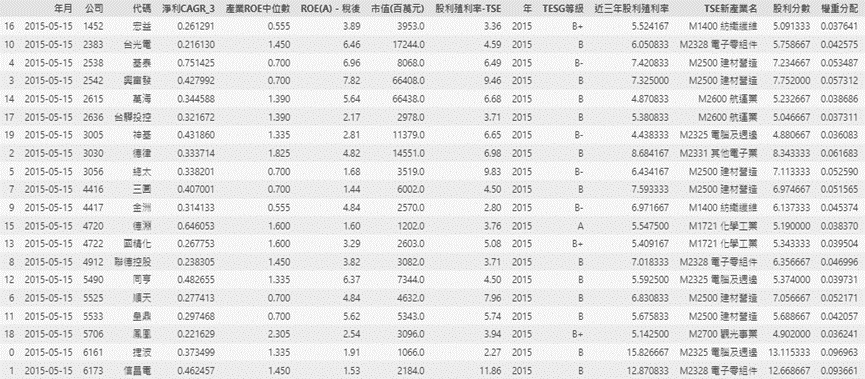
We integrate all screening criteria and calculation functions into the investment group formula in the table below. The parameter has an item year_2022, which assumes that the ESG scores of all stocks in 2022 are the same as those in 2021, so that we can observe the latest performance of the investment group.
def constr_index(n1, n2, n3, n4, init, tesg, year_2022=False):
    #Assuming 2022 ESG scores are the same as 2021
    tmp = tesg.loc[tesg['年'] == 2021].copy()
    tmp['年'] = 2022
    tesg = pd.concat([tesg, tmp]).reset_index(drop=True)
    #--------------------------------------------------------Selective enable

    fin_ind['常續性稅後淨利'].fillna(1)
    fin_ind['淨利CAGR_3'] = fin_ind.groupby('公司')['常續性稅後淨利'].transform(lambda x: (x.pct_change(n1) + 1)**(1/n1)-1 )

    fin_ind['產業ROE中位數'] = fin_ind.groupby(['年月', 'TSE新產業名'])['ROE(A)-稅後'].transform(lambda x: x.median())

    filter1 = pd.merge_asof(fin_ind.sort_values('年月'), price.sort_values('年月'), on='年月', by='公司').sort_values(['年月', '公司'])

    filter1['近三年股利殖利率'] = filter1.groupby('公司')['股利殖利率-TSE'].transform(lambda x: x.rolling(n2).mean())

    filter1 = filter1.merge(tesg, left_on=['年', '公司'], right_on=['年', '證券代碼'])

    filter1 = filter1[['公司', '代碼', '年月', '淨利CAGR_3', '產業ROE中位數', 'ROE(A)-稅後', '市值(百萬元)', '股利殖利率-TSE', '年', 'TESG等級', '近三年股利殖利率', 'TSE新產業名']]

    #Multi-point ROE Filter
    condition1 = filter1['淨利CAGR_3'] >= n3
    condition2 = filter1['ROE(A)-稅後'] >= filter1['產業ROE中位數']
    condition3 = filter1['市值(百萬元)']/100 >= 10

    filter1 = filter1[condition1 & condition2 & condition3]

    filter1['股利分數'] = filter1['近三年股利殖利率']*0.8 + filter1['股利殖利率-TSE']*0.2

    filter1 = filter1.dropna(subset=['股利分數'])

    div_30_Q = filter1.groupby('年月').apply(lambda x: x.nlargest(n4, '股利分數'))

    div_30_Q = div_30_Q.drop(columns=['年月']).reset_index().drop(columns='level_1')

    div_30_Q['權重分配'] = div_30_Q.reset_index().groupby('年月')['股利分數'].apply(lambda x: x/x.sum())
    #Adjustments are made in March and September every six months
    if year_2022 == False:
        div_30_Sem = div_30_Q[~(div_30_Q['年月'].dt.year == 2022)].sort_values(['年月', '公司'])  #~(div_30_Q['年月'].dt.month.isin([3, 8])) &
    else:
        div_30_Sem = div_30_Q.sort_values(['年月', '公司'])

    return cul_index(price, div_30_Sem, init), filter1, div_30_Sem
df, index_filter, div_30_Sem = constr_index(4, 12, 0.2, 20, 1000, tesg, year_2022=True)
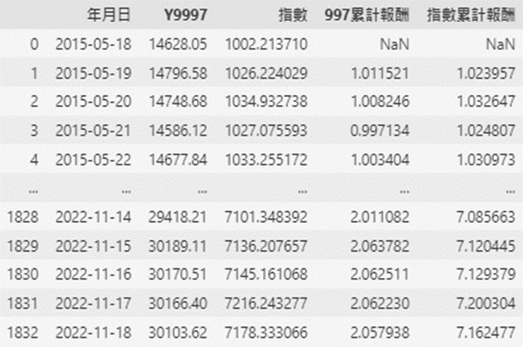
The parameters are the recurring net profit after tax in the past four quarters, the dividend yield rate in the past three years, the recurring net profit after tax CAGR >= 20%, 20 constituent stocks, a starting value of 1,000 points, and the assumption of starting the ESG score in 2022. As can be seen from the table below, a total of 30 rebalancings were carried out from May 2015 to November 2022, and the index grew from 1,000 points to 7,000 points.

We download the cumulative return index of the market during the same period – Y9997 as a control group to see if it can outperform the market. Obviously, compared with the 205% cumulative return of the broader market, our investment group outperformed the broader market with a cumulative return of 716%.
base_index = tej.get('TWN/APRCD1',
            coid=['y9997'],
            mdate={'gt': '2015-03-01', 'lt':'2022-12-01'},
            opts={'columns': ['coid', 'mdate', 'close_adj']},
            chinese_column_name=True,
            paginate=True)

base_index['年月日'] = base_index['年月日'].astype('datetime64[ns]')

base_index = base_index.pivot(columns='證券代碼', index='年月日', values='收盤價(元)').rename_axis(None, axis=1).reset_index()

result = base_index.merge(df, left_on='年月日', right_on='年月')

result['997累計報酬'] = (result['Y9997'].pct_change()+1).cumprod()
result['指數累計報酬'] = (result['指數'].pct_change()+1).cumprod()
result
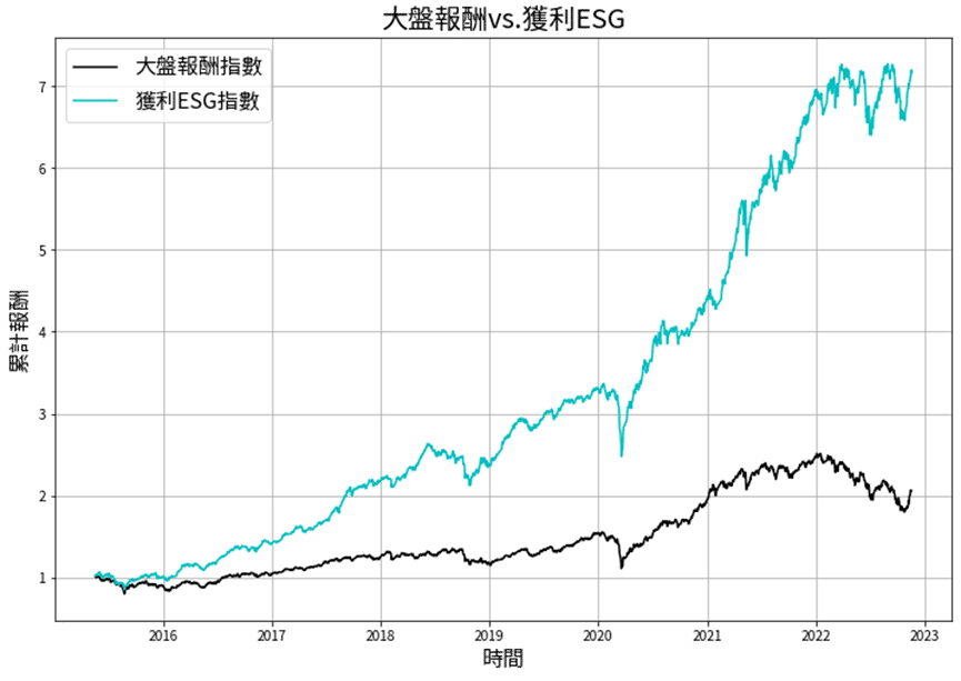
From the chart below, it can be clearly seen that the investment group has gradually widened the gap with the market since 2016. The largest increase came from the V-shaped reversal of the epidemic in 2020. Basically, the accumulated return rate for the year was close to 100%.
Calculate various common performance indicators such as rate of return, Sharpe value and MDD, etc.
stat = pd.DataFrame(index=['Y9997', '指數'],
                    columns=['年化標準差', '年化報酬率', '夏普值', 'MDD'],
                    data=[[cul_std(result['Y9997']), cul_ret(result['997累計報酬']), 0, mdd(result['997累計報酬'])],
                    [cul_std(result['指數']), cul_ret(result['指數累計報酬']), 0, mdd(result['指數累計報酬'])]])

stat['夏普值'] = stat['年化報酬率'] / stat['年化標準差']

stat['風報比'] = 0
stat['風報比'].iloc[0] = (result['997累計報酬'].iloc[-1]-1) / -stat['MDD'].iloc[0]
stat['風報比'].iloc[1] = (result['指數累計報酬'].iloc[-1]-1) / -stat['MDD'].iloc[1]
From the actual performance indicators, it can be seen that while far outperforming the market, the annualized standard deviation is only 0.18% higher than the market, and even the largest drawdown is only 26.45%, which is more stable than the market, and the wind report ratio is as high as 23.3.

Graphically presents the periodic retracement range of investment groups and the market.
fig, ax = plt.subplots(figsize=(20, 6))

plt.rcParams['font.sans-serif'] = ['Taipei Sans TC Beta']

ax.plot(result['年月日'], result['997累計報酬'].to_drawdown_series().to_list(), color='black', linewidth=1.5)

ax.fill_between(result['年月日'], np.zeros(len(result['997累計報酬'])), result['997累計報酬'].to_drawdown_series().to_list(), label='大盤 DD', color='black', linewidth=1, alpha=0.5)

ax.plot(result['年月日'], result['指數累計報酬'].to_drawdown_series().to_list(), color='blue', linewidth=1.5)

ax.fill_between(result['年月日'], np.zeros(len(result['指數累計報酬'])), result['指數累計報酬'].to_drawdown_series().to_list(), label='獲利ESG DD', color='c', linewidth=1, alpha=0.7)

ax.grid()

ax.legend(loc='best', fontsize=16)

plt.xlabel('時間', fontsize=16)
plt.ylabel('下跌幅度', fontsize=16)

plt.title('大盤報酬&獲利ESG 回撤幅度', fontsize=20)

plt.show()
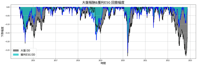
The table below shows the magnitude of the retracement compared with the broader market during the same period. It can be seen that although our blue investment group has been deeper than the broader market in the stock market declines in previous major events, it has been affected by the epidemic in 2020 and the big interest rate hike in the United States in 2022. The magnitude of the retracement is smaller than that of the market.
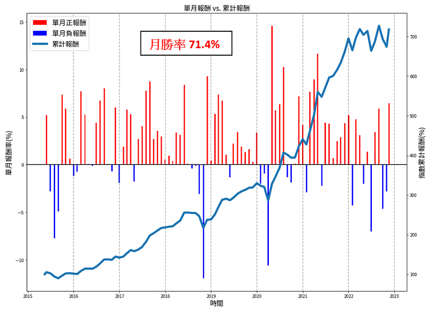
Graphical presentation of monthly positive and negative return distribution and cumulative rate of return.
fig = plt.figure(figsize=(16, 12))

ax = fig.subplots()

ax2 = ax.twinx()

ax.bar(index_m.index, [i if i >= 0 else 0 for i in index_m['單月報酬']], color='red', width=10, label='單月正報酬')

ax.bar(index_m.index, [i if i < 0 else 0 for i in index_m['單月報酬']], color='blue', width=10, label='單月負報酬')

ax2.plot(index_m.index, index_m['指數累計報酬']*100, label='累計報酬', linewidth=5)

ax.axhline(y = 0, color='black')

for i in range(2015, 2023):
    plt.axvline(x = [pd.Timestamp(i,12,31)], color='black', linestyle="--", alpha=0.3)

ax.set_xlabel('時間', fontsize=16)

ax.set_ylabel('單月報酬率(%)', fontsize=16)

ax2.set_ylabel('指數累計報酬(%)', fontsize=16)

plt.title('單月報酬 vs. 累計報酬', fontsize=16)

fig.legend(loc='upper left', bbox_to_anchor=(0,1), bbox_transform=ax.transAxes, fontsize=16)
If we take a closer look at the distribution of positive and negative returns every month, we can see that except for the 2018 Sino-US trade war, 2020 new coronavirus pneumonia, 2021 Taiwan epidemic, and 2022 Ukraine-Russia war & FED’s big interest rate hike, the basic monthly returns are mostly positive. Overall The monthly winning rate came to 71.4%.
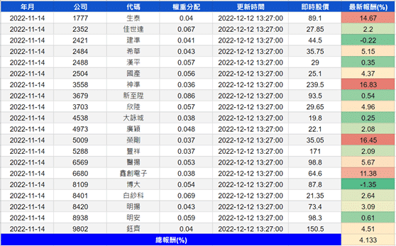
The most recent investment group screened the 20 constituent stocks in the table below. It can be seen that in the past month since November 14, at least 4 stocks with a return rate of more than 10% have been screened out, and the largest drop is only -1.35%. , the current rate of return came to 4.133%.
We use the ESG ratings of individual stocks provided by TESG as the basis, combined with the more demanding profit growth indicators, hoping to find targets with both sustainable management and growth potential in the vast sea of stocks, and from the results we have successfully achieved To achieve this goal, it has earned a cumulative return rate that is more than 2 times that of the market while being more stable than the market, showing that even if the investment portfolio incorporates ESG indicators, it can still obtain significant excess returns. The investment code provided in the article is integrated in the form of a function, so that readers who want to further adjust the parameters can also refer to the method in the article to select other financial indicators to construct an exclusive ESG investment portfolio.
Finally, we would like to remind you again that the objects mentioned in this article are for illustrative purposes only and do not represent recommendations or suggestions for any financial products. Therefore, if readers are interested in related topics such as construction strategies, performance backtesting, research evidence, etc., they are welcome to purchase the solutions in TEJ E Shop. With a complete database, various tests can be easily completed.