Use python and TEJ database to execute event study

Table of Contents
Seasoned equity offerings is a common financing option for listed firms, and the purpose of it includes expansion of capital expenditures, retirement of debts and improvement of financial structure. However, previous literature has implied that this borrowing behavior tends to send negative signals to the market, leading to stock prices plummeting at the date of announcement.
Event study is a statistical method that analyzes the impact of important corporate events(M&A, SEO, stock buyback…) or economic shocks(regulation change, policy, macroeconomic conditions…) on firms’ value. Basically, event study consists of the following steps: event date confirmation, definition of estimation window and event window, calculation of abnormal return and statistical test. Therefore, this week, we will verify whether this negative announcement effect also happens in the Taiwan stock market by adopting the TEJ API database and event study approach !
We use Windows OS and Jupyter Notebook in this article
import tejapi
import pandas as pd
import numpy as np
import matplotlib.pyplot as plt
from sklearn.linear_model import LinearRegression
from scipy import stats
tejapi.ApiConfig.api_key = 'Your Key'
tejapi.ApiConfig.ignoretz = True
Note: sklearn.linear_model is used for regression;scipy is for statistical test
tse_stockssecurity = tejapi.get('TWN/ANPRCSTD',
mkt = 'TSE',
stypenm = '普通股',
opts = {'columns':['coid','mdate','stypenm','mkt']},
paginate = True,
chinese_column_name = True)
tse_stocks = security['證券碼'].tolist()
events = tejapi.get('TWN/ASTK1',
               x_mt_date = {'gte':'2019-01-01', 'lte':'2021-08-01'},
               opts = {'columns':['coid','cash','x_mt_date']},
               paginate = True,
               chinese_column_name = True)
This article will treat the date of resolution of shareholders’ meeting as event day. The event day falls between January 2019 ~ August 2020
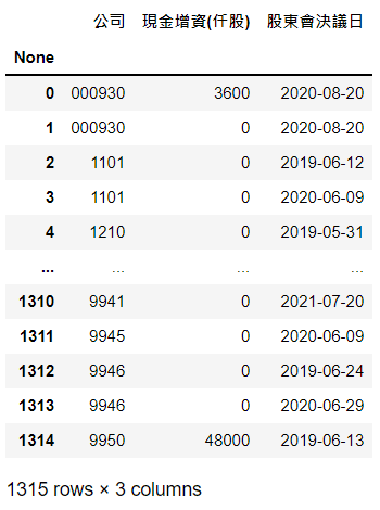
cash = events[events['現金增資(仟股)']>0].reset_index(drop=True)
We only need issuance of common stock for cash, instead of earnings or capital surplus transferred to common stock
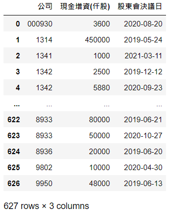
tse_cash = cash[cash['公司'].isin(tse_stocks)].reset_index(drop=True)
Combined with TSE-listed firms’ code tse_stocks and isin(),we finally obtain issuance of common stock for cash event only for TSE-listed firms tse_cash

Estimation window(T0~T1): -260~-10 periods is set. The actual returns in this period will be regressed on Fama & French factor-based portfolio return, which yields the coefficient estimates that will be used to calculate expected return within event window
Event day (0): the date of resolution of shareholders’ meeting, since it’s the earliest signal for SEO sent to market
Event window(T2~T3): -5 ~ +5 periods. The difference between actual return and expected return predicted by Fama & French model is so-called abnormal return
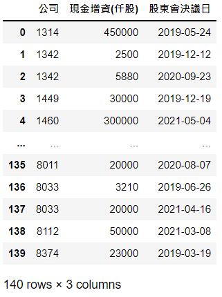
Because we include 140 events of common stocks issuance, each loop is used to cope with each event, and the output will be stored in variable final . We also exclude some events that lack data or belong to initial public offerings. In the following section, we select some important parts of codes within the loop to interpret and take the first event ( stock = ‘1314’, date = ‘2019–05–24’ ) as an example to show what’s going on in each loop. Other parts of codes can be viewed in source code
return_set = tejapi.get('TWN/APRCD',
                      coid = stock,
                      mdate = {'gte': date + pd.Timedelta(days =
                      -450), 'lte': date + pd.Timedelta(days = 25)},
                      opts = {'columns' : ['coid', 'mdate','roi']},
                      paginate = True,
                      chinese_column_name = True)
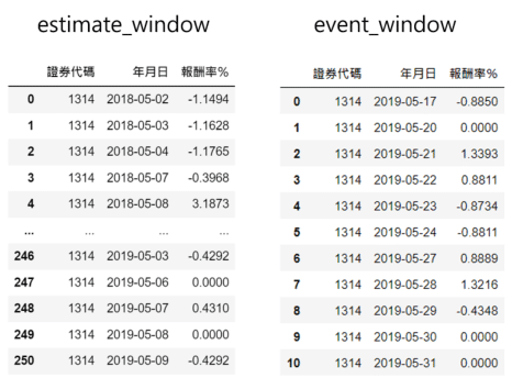
Each event has a unique combination of firm code stock and event date date , which are used to obtain return around event day. Here we choose the returns of 450 days before the event date and 25 days after the event date to make sure we’ll have complete return in estimation window(251 trading days) and event window(11 trading days)
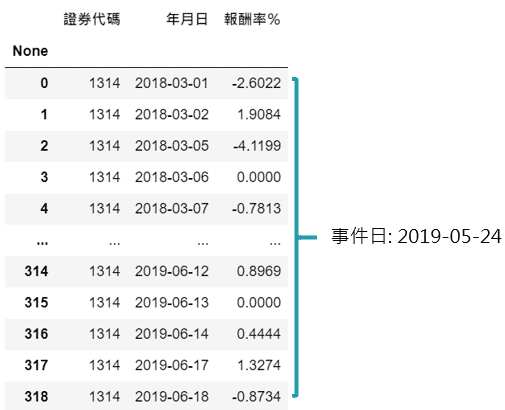
event_index = return_set[return_set['年月日'] == date].index.values.astype(int)[0]
First of all, the event date’s index should be used as a basis to split two windows
estimate_window = return_set[event_index - 260 - 1: event_index - 10].reset_index(drop=True)
event_window = return_set[event_index - 5: event_index + 5 + 1].reset_index(drop=True)
#估計起始日期(-260)
estimate_start = estimate_window.loc[0, '年月日']
#事件結束日期(+5)
event_end = event_window.loc[5*2, '年月日']
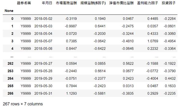
For starters, we need to find the beginning date of the estimation window and the last date of the event window. Then based on the two dates, we directly obtain the daily portfolio return of market risk premium, size premium, book-to-market premium, profitability and investment factors. Y9999 means the above returns are based on TSE-listed firms and belong to simple return
fama_french = tejapi.get('TWN/AFACTO1D',
                   coid = 'Y9999',
                   mdate = {'gte':estimate_start, 'lte': event_end},
                   opts = {'columns': ['coid',
                   'mdate','mrp','smbn','bp','op','inv']},
                   paginate = True,
                   chinese_column_name = True)
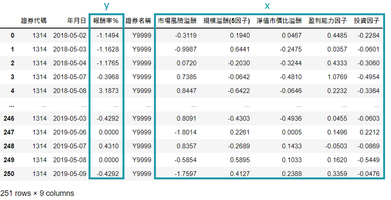
ols_data = estimate_window.merge(fama_french, on = '年月日')
x = ols_data.loc[:,['市場風險溢酬', '規模溢酬(5因子)','淨值市價比溢酬','盈利能力因子','投資因子']].values
y = ols_data['報酬率%'].values.reshape(-1,1)
model = LinearRegression()
model.fit(x,y)
After combining estimation return and Fama-French portfolio return, we convert them into two-dimensional array variables which are required in a linear model. Finally, put dependent variable and independent variable in the model
predict_data = event_window.merge(fama_french, on = '年月日')
event_x = predict_data.loc[:,['市場風險溢酬','規模溢酬(5因子)','淨值市價比溢酬','盈利能力因子','投資因子']].values
Here we combine the event window return with Fama & French portfolio return, and store the factor-based portfolio returns to be independent variables to get the expected return by putting them in fitted model model.predict() . The next step is to calculate the abnormal returns, cumulative returns and add one more columns to indicate the relative day
event_window['預期報酬率'] = model.predict(event_x)
event_window['異常報酬率'] = event_window['報酬率%'] - event_window['預期報酬率']
event_window['累計異常報酬率'] = event_window['異常報酬率'].cumsum()
event_window['相對天數'] = [i for i in range(-5, 5 + 1)]
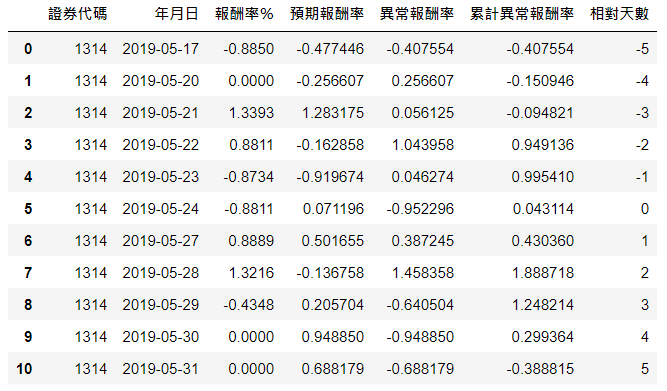
Each loop will keep repeating the above steps and the output will be added in final table, as the following shown
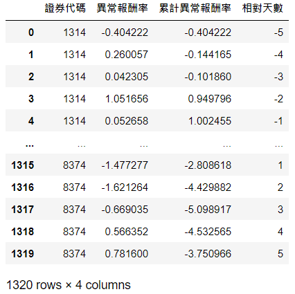
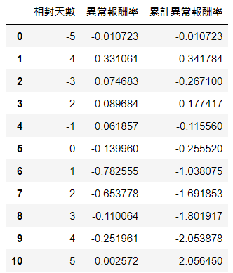
sorted_data = final.groupby(by = '相對天數').mean().reset_index()
plt.plot(sorted_data['相對天數'], sorted_data['異常報酬率'], label = 'Average Abnormal Retrun')
plt.plot(sorted_data['相對天數'], sorted_data['累計異常報酬率'], label = 'Cumulative Abnormal Return')
plt.xlabel('Event Day')
plt.title('Event Study')
plt.xticks(np.arange(-5, 5+1 , 1))
plt.legend()
plt.show()
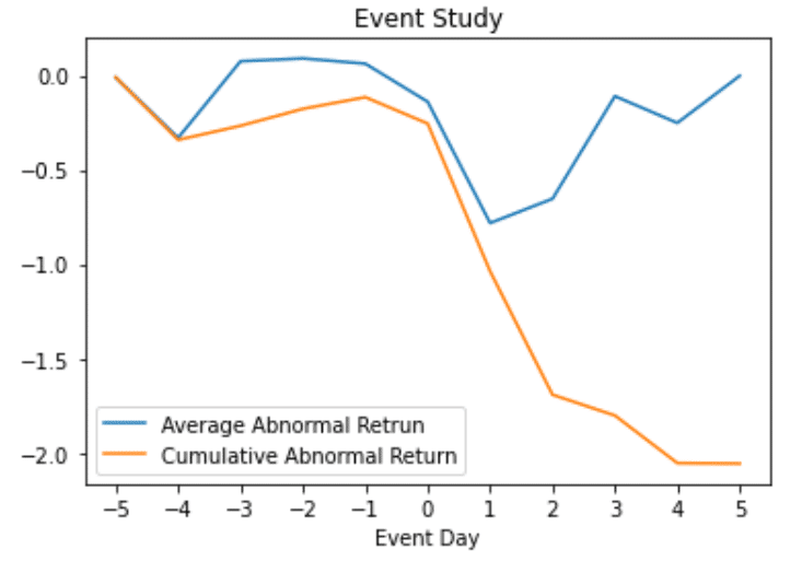
As you can see, there’s apparently negative abnormal return one or two days after the event day. However, the abnormal return reverses back around zero afterwards, which imply the market might already digest the information
ttest = pd.DataFrame()
for day in range(-5,5+1):
    sample = final[final['相對天數'] == day]['異常報酬率'].values
    t, p_value = stats.ttest_1samp(sample, 0)
    if p_value <= 0.01:
        significance = '***'
    elif 0.01 < p_value <= 0.05:
        significance = '**'
    elif 0.05 < p_value <= 0.1:
        significance = '*'
    else:
        significance = ''
    ttest = ttest.append(pd.DataFrame(np.array([day,t,p_value, significance]).reshape((1,4)), columns = ['相對天數','T檢定值', 'P-value','顯著水準'],)).reset_index(drop=True)ttest = ttest.set_index('相對天數')
We use stats.ttest_lsamp() to carry out T-tests to examine whether the daily abnormal return is significantly different from zero. We also add one more significance star column based on p-value
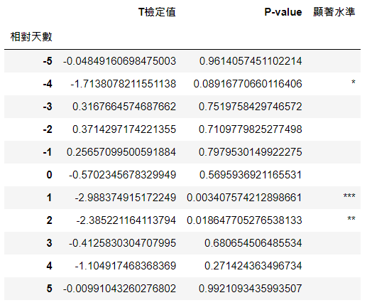
Therefore, we can prove that the announcement of SEO does significantly impact firms’ value. The reason for not impacting the return at the event date may result from firms usually declaring important issues after the stock market closes
After today’s introduction, we believe readers have more understanding of event study! Actually still lots of assumptions we proposed in this article can be adjusted based on previous literature or event characteristics, such as estimation and event window or the methods to calculate the abnormal return. To execute event study more efficiently, we highly recommend TEJ API databases as we use in this article given its quality and variety without wasting time on data crawling and cleaning. If readers are interested in observing other events’ impact on firms’ value, welcome to the TEJ E Shop to purchase the data that satisfy your need!