
KD indicator is one of the commonly-used indicators in technical analysis. It’s mainly used for judging the current strength of stock price or possible timing of reversing. Following is the way to calculate this indicator
- RSV = ((today’s closed price — lowest price in past N days)/(highest price in past N days — lowest price in past N days))*100
- K = yesterday’s K* (2/3) + today’s RSV*(1/3)
- D = yesterday’s D* (2/3) + today’s K*(1/3)
By observing the formula, we can interpret RSV as the strength of stock price in past N days (we use N=9 in this article). K is also called “fast line”, since it’s highly sensitive to today’s stock price; while D, obtained by using K, is less sensitive given its second smoothing calculation. In this article, we use following strategy to backtesting
Windows OS and Jupyter Notebook
#基本功能
import pandas as pd
import numpy as np
import copy
#繪圖
import plotly.graph_objects as go
import plotly.express as px
#TEJ
import tejapi
tejapi.ApiConfig.api_key = 'Your Key'
tejapi.ApiConfig.ignoretz = True
Table of Contents
Step 1. Obtain the stock price
stock_data = tejapi.get('TWN/APRCD',
                  coid= '2002',
                  mdate={'gte': '2021-01-01'},
                  opts={'columns': ['coid', 'mdate', 'open_d', 'close_d']},
                  chinese_column_name=True,
                  paginate=True)
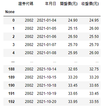
We choose China Steel Corporation (2002) as an example and the columns include opening price, which is used to calculate buying and selling price, and closing price that will produce buy and sell signal.
kd_data = copy.deepcopy(stock_data)
#設9天
kd_data['9_high'] = kd_data['收盤價(元)'].rolling(9).max()
kd_data['9_low'] = kd_data['收盤價(元)'].rolling(9).min()
#rsv
kd_data['rsv'] = ((kd_data['收盤價(元)']-kd_data['9_low'])/(kd_data['9_high']-kd_data['9_low']))*100
kd_data['rsv'] =  kd_data['rsv'].fillna(50)
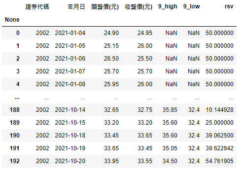
Since we need a clean stock_data later on, we use deepcopy() to copy its content to variable kd_data. Then get the highest and lowest closed price over the past 9 days. Finally, RSV can be calculated and the missing value is filled with 50
#初始化kd與買賣股數
kd_data['k'] = 0
kd_data['d'] = 0
kd_data['買賣股數'] = 0
#迴圈修正k d值
hold = 0
for i in range(len(kd_data)):
    #先算出當期的k d 值
    if i == 0:
        kd_data.loc[i,'k'] = 50
        kd_data.loc[i,'d'] = 50
    else:
        kd_data.loc[i,'k'] = (2/3* kd_data.loc[i-1,'k']) + (kd_data.loc[i,'rsv']/3)
        kd_data.loc[i,'d'] = (2/3* kd_data.loc[i-1,'d']) + (kd_data.loc[i,'k']/3)

    if kd_data.loc[i, 'k'] <= 20:
        if hold == 0:
            kd_data.loc[i+1, '買賣股數'] = 1000
            hold = 1
    elif kd_data.loc[i,'k'] >= 80:
        if hold > 0:
            kd_data.loc[i+1,'買賣股數'] = -1000
            hold = 0
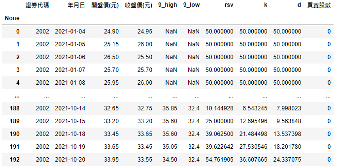
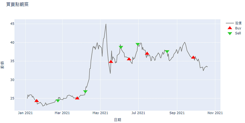
After initializing KD and trading shares, we get into the loop to calculate KD that we need to produce signals for buy and sell. Because current KD is based on previous KD values, we have to set the first KD as 50 by default. Then hold represents whether we hold the shares (1 = Yes, 0=No). If buy signal(K≤20) is met and we have no stocks on hand, we’ll buy 1000 shares at the opening of next day. On the other side, if sell signal (K≥80) is satisfied and we have some shares, then sell it next day at the opening price.
In 【Quant(8)】Backtesting by MACD Indicator, we have discussed the details in the calculation of frictions cost and the method to calculate return with initial principal. In this article, we use function to achieve all of it.
def ret(data, principal):

    #計算成本
    data['手續費'] = data['開盤價(元)']* abs(data['買賣股數'])*0.001425
    data['手續費'] = np.where((data['手續費']>0)&(data['手續費'] <20), 20, data['手續費'])
    data['證交稅'] = np.where(data['買賣股數']<0, data['開盤價(元)']* abs(data['買賣股數'])*0.003, 0)
    data['摩擦成本'] = (data['手續費'] + data['證交稅']).apply(np.floor)

    #計算資產價值
    data['股票價值'] = data['買賣股數'].cumsum() * data['收盤價(元)']
    data['現金價值'] = principal - data['摩擦成本'] + (data['開盤價(元)']* -data['買賣股數']).cumsum()
    data['資產價值'] = data['股票價值'] + data['現金價值']

    #計算報酬率
    data['當日價值變動(%)'] = (data['資產價值']/data['資產價值'].shift(1) - 1)*100
    data['累計報酬(%)'] = (data['資產價值']/principal - 1)*100

    return data
With the data containing trading shares and initial principal, we can quickly get the transaction costs and return. In this article, we set 30,000 as our principal
kd_return = ret(data = kd_data, principal = 30000)
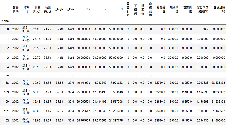
Besides, to demonstrate whether this strategy performs relatively well, we add buy-and-hold strategy and market performance as our benchmarks
bh_data = copy.deepcopy(stock_data)
bh_data['買賣股數'] = 0
bh_data.loc[0, '買賣股數'] = 1000
bh_data.loc[len(bh_data)-1, '買賣股數'] = -1000
bh_return = ret(data=bh_data, principal = 30000)
Here we also use deepcopy() to get stock price, and choose to buy at the beginning and sell at the end during the same period with initial principal of 30000.
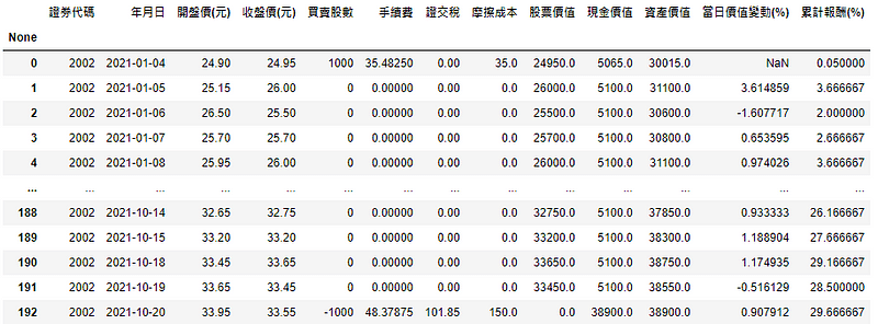
market = tejapi.get('TWN/APRCD',
                    coid = 'Y9997',
                    mdate = {'gte':'2021-01-01'},
                    opts = {'columns':['coid','mdate', 'roi']},
                    chinese_column_name = True)
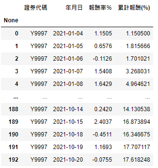
market['累計報酬(%)'] = (market['報酬率%'].apply(lambda x:0.01*x +1).cumprod() - 1)*100
Obtain return of market return index (Y9997) to stands for market performance and calculate the cumulative return
Step 1. Comparison of cumulative return (See the details in source code)
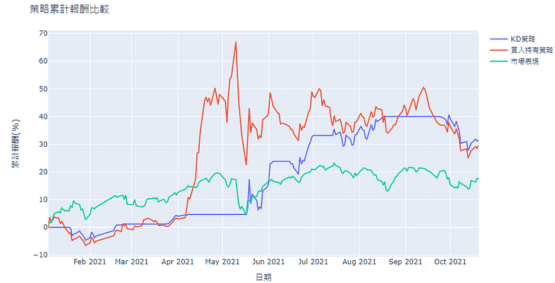
Here we can see this year’s market performance is relatively weak. The return of buy-and-hold strategy basically follows the stock price, thereby benefitting from upside trend in May. And KD strategy considers not only the stock price, but also positions. For example, there’s no change in cumulative return in May because we hold no stocks in hand and only have cash positions, leading to missing the strong bullish trend.
Step 2. Performance table (See the details in source code)
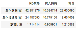
Although annualized return of KD and buy-and-hold strategy are quite similar, KD appears to be better than others after taking the risk into consideration
After reading this article, we believe readers can better understand the definition and limitations of KD indicator. For instance, when stock market seems overly optimistic, the sell signal will pop up. However, if the bullish market remains for quite a long time, using KD strategy to exit the market may not be a smart choice. Overtrading, causing lots of friction costs, may be the common issue in technical analysis that drags down its cumulative return. At the end, its performance may even be worse than just buy-and-holding! Thus, other indicators are still needed to make more proper judgement of buying and selling. If readers are interested in this kind of technical analysis backtesting, welcome to purchase the plan offered in TEJ E-Shop, since we all know data of higher quality is the important foundation of the closest-to-real-world backtesting.