Use TEJ API to construct our own backtest system.

Table of Contents
Trade Backtest is a more scientific approach to test strategy nowadays. Although the past cannot represent the future. The result of backtest can provide us some information about the strategy. However, if we have to run different strategy, we need to build a new system. This way will waste our much time and it is inefficient. Therefore, we try to modular the system and focus on developing the strategy.
We use Windows OS and Jupyter Notebook in this article.
import tejapi
import pandas as pd
import numpy as np
tejapi.ApiConfig.api_key = 'Your Key'
tejapi.ApiConfig.ignoretz = True
Note: Remember to replace ‘Your key’ with the one you applied for. The last line indicates that we ignore the time zone.
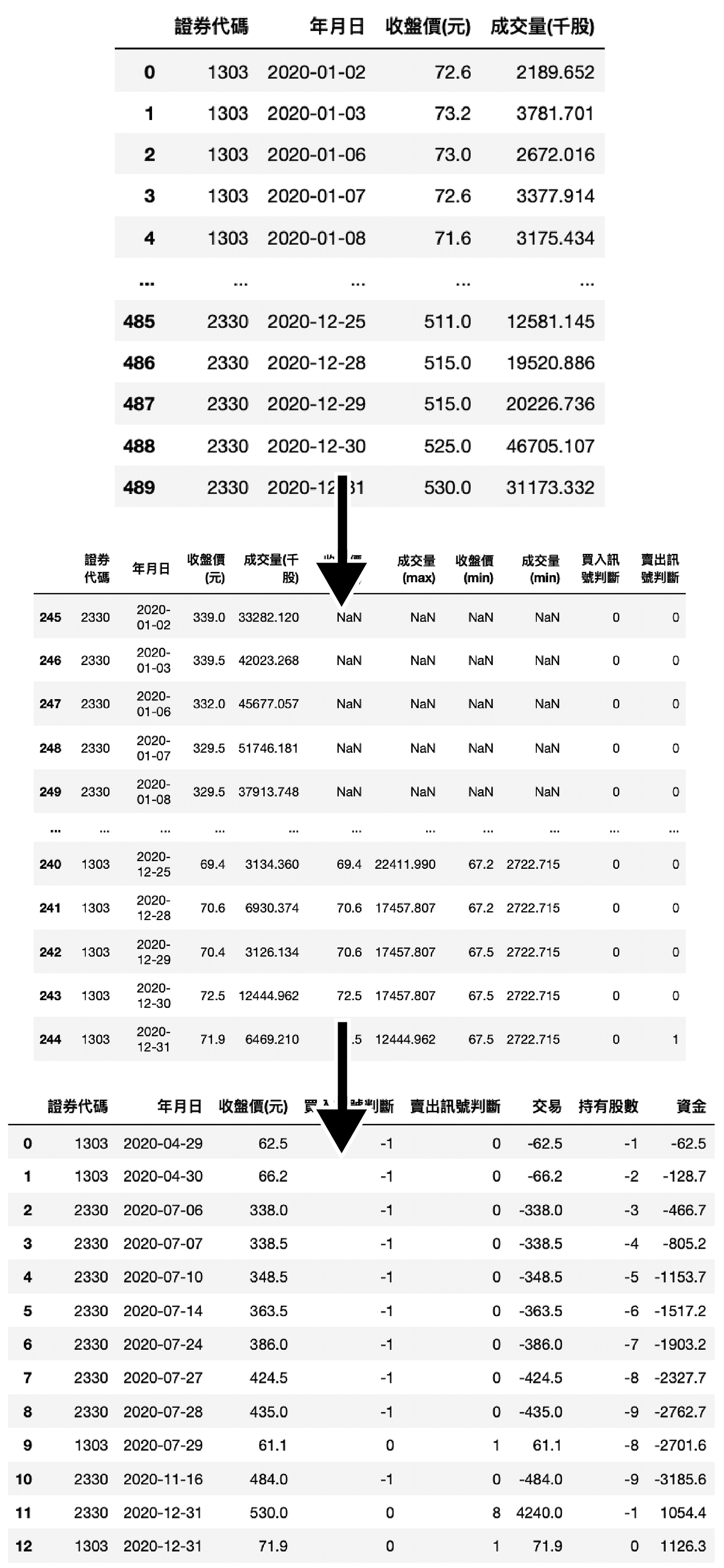
Consider the columns required for the process.
class name backtestclass backtest():def is created under this class.def __init__(self, target_list):
# 設定初始值
# 股票池
self.target_list = target_list
# 訊號表
self.signal_data = pd.DataFrame()
# 交易表
self.action_data = pd.DataFrame()
# 獲利數
self.protfolio_profit = []
# 成本數
self.protfolio_cost = []Raw also need to put it into this class. target_list is our stock pool.
# 資料庫
self.data = tejapi.get('TWN/APRCD',
               coid = target_list,
               mdate={'gte':'2020-01-01', 'lte':'2020-12-31'},
               opts={'columns':['coid','mdate','close_d',
               'volume']},
               chinese_column_name=True,
paginate=True).reset_index(drop=True)We will buy the stock if the price and volume break through the highest price and volume in the past 20 days.
def price_volume(self, specific=None):
        # 策略更新
        self.signal_data = pd.DataFrame()
        self.action_data = pd.DataFrame()
Generate transaction signals for each stock.
# 股票池每一檔股票都跑一次訊號產生
 for i in self.target_list:
    target_data = self.data[self.data['證券代碼'] == i]
Calculate the highest and lowest price and volume in past 10 and 20 days.
rolling_max = target_data[['收盤價(元)', '成交量(千股)']].rolling(20).max()rolling_min = target_data[['收盤價(元)', '成交量(千股)']].rolling(10).min()
Buy
stock_data['買入訊號判斷'] = np.where((stock_data['收盤價(元)'] == stock_data['收盤價(max)']) & (stock_data['成交量(千股)'] == stock_data['成交量(max)']), -1, 0)Sell
stock_data['賣出訊號判斷'] = np.where((stock_data['收盤價(元)'] == stock_data['收盤價(min)']) & (stock_data['成交量(千股)'] == stock_data['成交量(min)']), 1, 0)Offset on last day
remain_stock = self.signal_data.iloc[:-1,8:10].sum().sum()
self.signal_data.iloc[-1,9] = 0
self.signal_data.iloc[-1,8] = 0
if remain_stock < 0:
    self.signal_data.iloc[-1,9] = -remain_stock
else:
    self.signal_data.iloc[-1,8] = -remain_stock
def buy_hold(self, specific=None):
        # 策略更新
        self.signal_data = pd.DataFrame()
        self.action_data = pd.DataFrame()
Generate transaction signals for each stock.
# 股票池每一檔股票都跑一次訊號產生
 for i in self.target_list:
    target_data = self.data[self.data['證券代碼'] == i]
Buy on first day and Sell on last day
target_data['買入訊號判斷'] = 0
target_data['賣出訊號判斷'] = 0

# 第一天買入,最後一天賣出
target_data.iloc[0, 4] = -1
target_data.iloc[-1,5] = 1def run(self, specific=None):
# 做出交易紀錄表
trade_data = pd.DataFrame(index= self.data['年月日'], columns=self.target_list).fillna(0.0)
action_data = self.signal_data[(self.signal_data['買入訊號判斷'] != 0) | (self.signal_data['賣出訊號判斷'] != 0)]Calculate Profit
# 計算個股總獲利
        self.protfolio_profit.append(sum(action_data['交易'].tolist()))
Calculate Cost
# 計算個股總成本
self.protfolio_cost.append(-action_data[action_data['買入訊號判斷'] < 0]['交易'].sum())def ROI(self):
# 報酬率
return_profit = sum(self.protfolio_profit) /
sum(self.protfolio_cost)
return return_profit
We usually compare our strategy to market return. That is because we want beat the market to obtain excess profits.
Step 1. Creating class name market, here we use ‘Y9997’ to represent market index.
market = backtest(['Y9997'])market.buy_hold()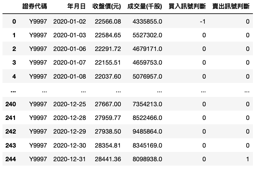
market.run()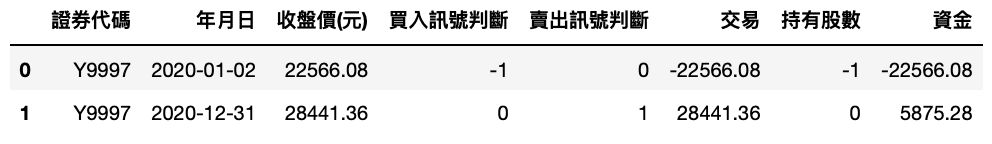
market.ROI()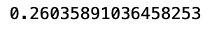
Now we want to use MSCI to be our portfolio. MSCI is an acronym for Morgan Stanley Capital International. It is an investment research firm that provides stock indexes, portfolio risk and performance analytics. Code of Database is TWN/AIDXS , and we can find MSCI portfolio in 2020.
data_MSCI = tejapi.get('TWN/AIDXS',
                       coid = 'MSCI',
                       mdate= '2019-12-31',
                       opts={'columns':['coid','mdate','key3']},
                       chinese_column_name=True)
Filter the data and save it to the list.
MSCI_list = data_MSCI['成份股'].unique().tolist()Delete the Chinese name.
MSCI_list = [coid[:4] for coid in MSCI_list]
Due to the effect of module, we do not need to rewrite the process of backtest. Just need to change target_list to get the result we want.
class name msci , target_list is MSCI_list.msci = backtest(MSCI_list)msci.price_volume()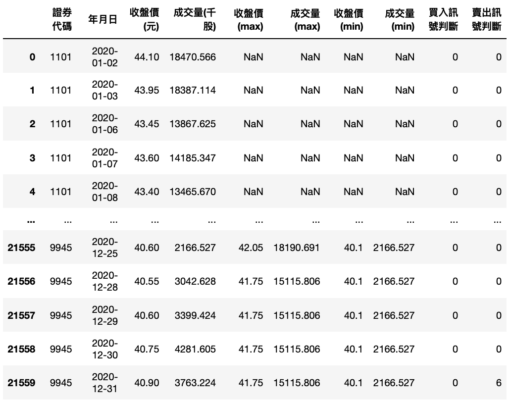
msci.run()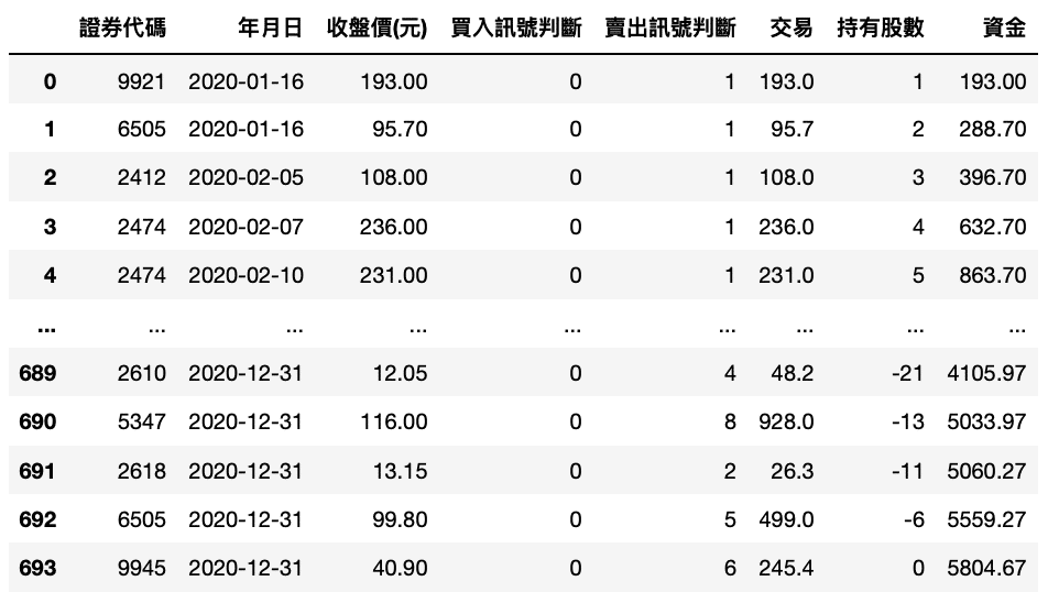
msci.ROI()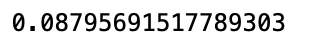
There will be a strong bull market in Taiwan’s stock market in 2020. It seems like buy and hold is better than price_volume strategy. But the period just only one year, we cannot jump to conclusion that which is better one. Today’s article describes how to build a simple backtest system. Reader can try to adjust the structure. For example, turn rolling days 10 、20 into adjustable parameters, in order to compare the compact of date change on the rate of return.
Quantitative Analysis is the trend of investment. Worldwide famous hedge fund adopt this method to make trade strategy. If you have interest on this topic, you can go to our official website. It provides various financial data to help you make better strategy.
