
Using NumPy and Pandas to start your first step of data analysis
After reading our previous articles, you might have already known how to get the data from TEJ API, store it into your computer, and update automatically! Then we are going to tell you how to analyze this data by using these two important packages- Numpy and Pandas
Table of Contents
Numpy is designed to conveniently and efficiently process n-dimensional and large-scale data arrays. With built-in functions, users could perform preliminary and rapid data processing.
import numpy as np
a = np.array([0, 0.5, 1.0, 1.5, 2.0]) #float ndarray -1-1.
b = np.array(['a', 'b', 'c']) #string ndarray        -1-2.
c = np.arange(0, 10, 2) #array([0, 2, 4, 6, 8])      -2.
c[2:] #array([4, 6, 8])                              -3.
c[:2] #array([0, 2])                                 -4.
Examples above:
a = np.arange(0, 30, 2) #array([0, 2, 4, ..., 28])
a.sum() #210                                      -1-1.
a.mean() #14.0                                    -1-2.
a.std() #8.640987                                 -1-3.
a.cumsum() #array([0, 2, 6, 12, ...,210])         -1-4.
lst = [0, 2, 4]
lst*2 = [0, 2, 4, 0, 2, 4]                        -2-1.
a+a #array([0, 4, 8, ..., 56])                    -2-2.
a*a #array([0, 4, 16, ..., 784])                  -2-3.
Examples above:
The first example is to use numpy built-in functions to calculate. In the second example, we can see the numpy vectorized computation. If we multiply a list(2–1) by 2, the number of elements in the list will double instead of doubling the value. But if it is numpy array(2–2, 2–3), it is possible to perform mathematical operations on the corresponding positions of the elements in the array~💪💪
b = np.array([a, a*2]) #array([0, 2, 4, ..., 28],
                              [0, 4, 8, ..., 56])
b[0] #array([0, 2, 4, ..., 28])                   -1-1.
b[0][1] #2                                        -1-2.
b.sum(axis = 1) #array([210, 420])                -1-3.
b.shape #(2, 15)                                  -2-1.
b.reshape(5,6) #array([0, 2, 4, 6, 8, 10],        -2-2.
                              ...
                      [36, 40,   ..., 56]])
Examples above:
Next, let’s take a look at how numpy performs on multi-dimensional arrays. Similarly, we also use “[]” to select. The difference is that there are more elements that can be selected, so we can use 2 “[][]” to select column and position respectively. If we want to do some matrix operations, we can use shape functions in numpy to check and find the desired shape to do the calculation.~💪💪
#boolean
b > 15    #array([False, False, ..., True],        -1-1.
                 [False, False, ..., True])
np.where(b>15, 1, 0) #array([0, 0, ..., 1],        -1-2.
                            [0, 0, ..., 1])
#random variable
np.random.normal(5, 2, 10)                         -2-1.
np.random.standard_normal(5)                       -2-2.
#financial
pip install numpy_financial
import numpy_financial as npf
npf.fv(0.03, 5, 0, -1000) #1159.27                 -3-1.
#fv(rate, nper, pmt, pv)
npf.irr([-95, 3, 3, 3, 103]) #0.0439               -3-2.
#irr(values)
Examples above:
Numpy has many applications for data processing, so it is very difficult for us to tell you all of them in just one article😢. Therefore, if you are interested in numpy, you can go through Numpy Official Website or leave the message below!💪💪
Pandas is a package that specializes in analyzing table data. Just like Excel, it presents data in a format we called DataFrame in order to help users analyze data more conveniently, especially for financial time series data.
import pandas as pd
df = pd.DataFrame([1, 2, 3, 4],
                  columns = ['Numbers'],
                  index = ['index_a','index_b','index_c','index_d'])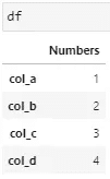
From the codes above, we can create a table with column name “Numbers” and row names ”index_a, b, c, and d” respectively.
df.loc['index_a'] #Numbers 1                                  -1-1.
df.iloc[0:2] #refer to source code                            -1-2.
df * 2 #same as numpy                                         -1-3.
#add "Name" column
df['Name'] = ['Amy', 'Bob', 'Catherine', 'Duke']              -2-1.
#select whole column
df['Numbers']                                                 -2-2.
#delete column
df.drop('column name', axis=1)                                -2-3.
#Math
df['Numbers'].sum() #10                                       -3-1.
df['Numbers'].mean() #2.5                                     -3-2.
df['Numbers'].std() #1.291                                    -3-3.
Examples above:
Like the numpy arrays which we have mentioned earlier, in Pandas, we also use brackets [“column name”] to select or add columns. But we will have to use the drop() function to delete columns. For operations, pandas dataFrame can perform basic statistical calculations in tables.~💪💪
import tejapi
tejapi.ApiConfig.api_key = “你的api_key”
df = tejapi.get('TWN/EWPRCD',
coid = ['2330'],
mdate={'gte':'2020-01-01', 'lte':'2020-12-31'},
opts={'columns': ['mdate','open_d','high_d','low_d','close_d']},
paginate=True
)
#Math
df.describe()
np.mean(df)
np.log(df)
#Plot
df['close_d'].plot()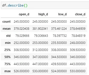
The sample data we used for pandas data analysis is 2330.TW stock price daily data got from the TEJ API. Then, most of the statistics that may be used further can be obtained through describe() function(figure above👆). If we want to do some operations on these values, we could directly use numpy to perform operations on the entire table!
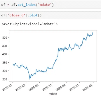
Last is the data visualization. There are several ways for users to plot the graph in python, and Pandas provides a very very easy one! If the chart we want to present is not complicated such as simple stock daily price, daily return, etc. We can select the column and use the plot() function to directly see the result! (figure above👆)
The only thing we have to note here is that the X and Y axes in the chart are the index and data you select respectively. That’s why we use a set_index() function to process our raw data at first.
What we share with you this time is how to use Numpy and Pandas packages to do the data analysis. However, it is very difficult for us to explain all the functions included in these 2 packages. Therefore, if you have any question or interested in any topic, you could go to their websites or leave the message below ❗️❗️ Then, we will go further into financial data analysis and applications in the next article, please look forward to it ❗️❗️
Finally, if you like this topic, please click 👏 below, giving us more support and encouragement. Additionally, if you have any questions or suggestions, please leave a message or email us, we will try our best to reply to you.👍👍
