Use market strength indicators cross strategy to backtesting
Table of Contents
Difficulty:★★☆☆☆
Use market strength indicators to do the moving average cross investment strategy
Advice:We use various technical indicators and strict long & short filter condition to judge the numbers of stocks strength and calculate market long short indicators. Using moving average cross strategy and visualization trading signal and buy sell point, then using optimal to get the best parameter.
By pulling up the weighted stocks like as TSMC, Media TEK to lead the market index rise, and others stocks fall. It will lead to investors who observe the market index have wrong judgement. We use strict long & short filter condition to construct market strength indicators and design a moving average cross strategy and use optimal to find the best parameter. The following strategies are used to backtesting and adjusted through optimization:
1. entry condition: 20 days moving average of day three lines short indicators more than 20 days moving average of day of three lines long indicators
2. leaving condition: 20 days moving average of day of three lines long indicators more than 20 days moving average of day three lines short indicators
This article uses Mac OS as system and jupyter as editor.
import pandas as pd
import numpy as np
import tejapi
import matplotlib.pyplot as plt
import matplotlib.transforms as transforms
from matplotlib.font_manager import FontProperties#Tej Api
tejapi.ApiConfig.api_key = "Your Key"
tejapi.ApiConfig.ignoretz = True
Security properties Data Table (TWN/ANPRCSTD)
No adjustment of(daily)technical indicators (TWN/AVIEW1)
Future database (TWN/AFUTR)
Due to the large amount of data, we divided it into multiple fetching from TEJ API.
data=tejapi.get('TWN/ANPRCSTD' ,chinese_column_name=True )
select=data["上市別"].unique()
select=select[1:3]
condition =(data["上市別"].isin(select)) & ( data["證券種類名稱"]=="普通股" )
data=data[condition]
twid=data["證券碼"].to_list()  #取得上市櫃股票證券碼
df = tejapi.get('TWN/AVIEW1', #從TEJ api撈取所需要的資料
                  chinese_column_name = True,
                  paginate = True,
                  mdate = {'gt':"2022-01-01", 'lt':'2022-08-31'},
                  coid=twid,
                  opts={'columns':['coid','mdate','close_d','kval','dval', 'dif','macd','a10ma']})
df1 = tejapi.get('TWN/AVIEW1', #從TEJ api撈取所需要的資料
                  chinese_column_name = True,
                  paginate = True,
                  mdate = {'gt':'2021-01-01', 'lt':'2022-01-01'},
                  coid=twid,
                  opts={'columns':['coid','mdate','close_d','kval','dval', 'dif','macd','a10ma']})df2 = tejapi.get('TWN/AVIEW1', #從TEJ api撈取所需要的資料
                  chinese_column_name = True,
                  paginate = True,
                  mdate = {'gt':'2020-01-01', 'lt':'2021-01-01'},
                  coid=twid,
                  opts={'columns':['coid','mdate','close_d','kval','dval', 'dif','macd','a10ma']})Y9999 = tejapi.get('TWN/AFUTR', #從TEJ api撈取所需要的資料
                  chinese_column_name = True,
                  paginate = True,
                  coid = 'ZTXA',
                  mdate = {'gt':'2020-01-01', 'lt':'2022-08-31'},
                  opts={'columns':['coid','mdate','close_d']})df3 = pd.merge(df2,df1,how='outer')
df4 = pd.merge(df3, df, how='outer') #將抓下來的技術指標合起來
df4.set_index(df4["日期"], inplace=True)
df4.drop(columns={'日期'}, inplace=True)
df4
We filter the day go long and go short stocks.
Long condition: K> D, diff> MACD, close>10 days moving average
Short condition: K<D, diff<MACD, close<10 days moving average
condition1 = (df4["K值"] > df4["D值"]) &(df4["差離值"]> df4["MACD"]) & (df4["收盤價"] > df4["10日移動平均"])#日三線多指標的條件
condition2 = (df4["K值"] < df4["D值"]) &(df4["差離值"] < df4["MACD"]) & (df4["收盤價"] < df4["10日移動平均"])#日三線空指標的條件long = df4[condition1] #把符合條件的篩選出來
short = df4[condition2]
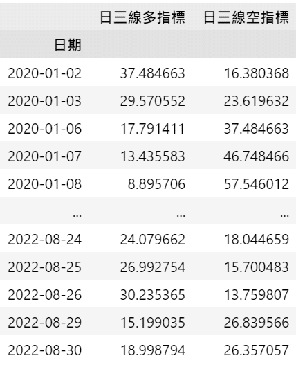
The number of stocks that correspond to go long condition divided by the number of samples and multiplied 100 to calculate day three lines long indicators.
The number of stocks that correspond to go short condition divided by the number of samples and multiplied 100 to calculate day three lines short indicators.
We merge the day three lines long indicators and the day three lines short indicators.
long1 = ((long.groupby('日期')['證券碼'].count())/(df4.groupby('日期')['證券碼'].count()))*100 #計算出日三線多指標
short1 =((short.groupby('日期')['證券碼'].count())/(df4.groupby('日期')['證券碼'].count()))*100 #計算出日三線空指標
long1.name = '日三線多指標' #重新命名
short1.name = '日三線空指標'
result = pd.concat([long1,short1], axis=1) #把兩表合併起來
We merge the market close price and long short indicators, then calculate 20 days moving average of day three lines long short indicators.
result1 = result.merge(Y9999[['日期', '收盤價']], on='日期')result1['日多20ma'] = result1['日三線多指標'].rolling(20).mean()
result1['日空20ma'] = result1['日三線空指標'].rolling(20).mean()result1.set_index(result1['日期'], inplace=True)
result1.drop(columns = {'日期'}, inplace=True)
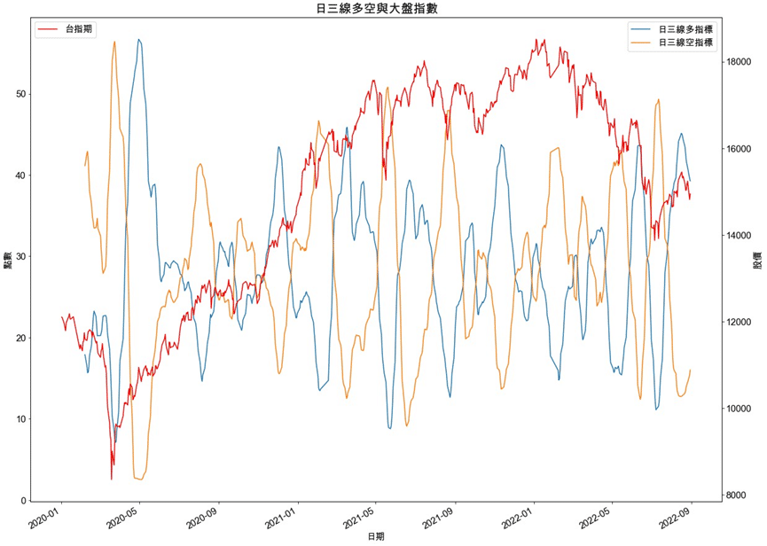
We draw out the picture to observe the situation, we can find that the day three lines long short indicators are more suitable for reverse strategy. Therefore, the previous entry and leave condition which is refer to the drawing result.
fig, ax1= plt.subplots(figsize =(20,16))
plt.plot(result1.index , result1['日多20ma'],lw=1.5, label = '日三線多指標')
plt.plot(result1.index , result1['日空20ma'],lw=1.5, label = '日三線空指標')
plt.xlabel('日期',fontsize=15)
plt.ylabel('點數', fontsize=15)
plt.xticks(fontsize=15)
plt.yticks(fontsize=15)
plt.title('日三線多空與大盤指數',  fontsize=20)
plt.legend(loc=1, fontsize=15)ax2 = ax1.twinx() #跟第一張ax1的x軸一樣
plt.plot(result1.index, result1['收盤價'] , lw=1.5, color='r', label='台指期')
plt.ylabel('股價', fontsize=15)
plt.yticks(fontsize=15)
plt.legend(loc=2, fontsize=15)plt.gcf().autofmt_xdate() #讓x軸的時間軸比較寬鬆、漂亮
plt.show()
We construct backtesting system and entry&exit point and write the signal and some common performance indicators into function, such as: the numbers of trades, average returns, cumulative returns, win rate and buy&hold returns. It’s convenient for investors to evaluate the trading strategy, and it can also be rewritten according to need. Among them, n1 and n2 are the parameter of the long short indicators, which can be adjusted about optimization later.
def buysell(data,n1,n2):
    data =data.copy()
    buy=[]
    sell=[]
    hold=0
    data['日多ma'] = data['日三線多指標'].rolling(n1).mean()
    data['日空ma'] = data['日三線空指標'].rolling(n2).mean()
    data.dropna(inplace=True)
    for i in range(len(data)):

        if  data["日空ma"][i] > data["日多ma"][i]:
            sell.append(np.nan)
            if hold !=1:
                buy.append(data["收盤價"][i])

                hold = 1
            else:
                buy.append(np.nan)
        elif data["日多ma"][i] > data["日空ma"][i] :
            buy.append(np.nan)
            if hold !=0:
                sell.append(data["收盤價"][i])
                hold = 0
            else:
                sell.append(np.nan)
        else:
            buy.append(np.nan)
            sell.append(np.nan)
    a=(buy,sell)

    data['Buy_Signal_Price']=a[0]
    data['Sell_Signal_Price']=a[1]
    data["買賣股數1"]=data['Buy_Signal_Price'].apply(lambda x : 1 if x >0 else 0)
    data["買賣股數2"]=data['Sell_Signal_Price'].apply(lambda x : -1 if x >0 else 0  )
    data["買賣股數"]=data["買賣股數1"]+ data["買賣股數2"]

    b = data[['Buy_Signal_Price']].dropna()
    c = data[['Sell_Signal_Price']].dropna()
    d = pd.DataFrame(index=c.index, columns = {"Buy_Signal_Price", 'Sell_Signal_Price'})
    for i in range(len(d.index)):
        d["Buy_Signal_Price"][i] = b["Buy_Signal_Price"][i]
        d['Sell_Signal_Price'][i] = c['Sell_Signal_Price'][i]
    d['hold_return'] = (d['Sell_Signal_Price']-d['Buy_Signal_Price'])/d['Buy_Signal_Price']
    win_rate = ((np.where(d['hold_return']>0, 1, 0).sum())/len(d.index))*100
    hold_ret = (d['hold_return'].sum())*100
    avg_ret = (d['hold_return'].mean())*100
    std = (d['hold_return'].std())*100

    final_equity = 10000
    for i in range(len(d.index)):
        final_equity = final_equity*(d['hold_return'][i]+1)
    cul_ret = ((final_equity-10000)/10000)*100
    y9999 = ((data['收盤價'][-1] - data['收盤價'][0])/data['收盤價'][0])*100

    #Visually show the stock buy and sell signal
    plt.figure(figsize=(20,16))
    # ^ = shift + 6
    plt.scatter(data.index,data['Buy_Signal_Price'],color='red', label='Buy',marker='^',alpha=1)
    #小寫的v
    plt.scatter(data.index,data['Sell_Signal_Price'],color='green', label='Sell',marker='v',alpha=1)
    plt.plot(data['收盤價'], label='Close Price', alpha=0.35)
    plt.title('買賣訊號', fontsize=20)
    #字斜45度角
    plt.xticks(rotation=45)
    plt.xlabel('Date', fontsize=15)
    plt.ylabel('Price',fontsize=15)
    plt.yticks(fontsize=15)
    plt.xticks(fontsize=15)
    plt.legend(fontsize=15)
    plt.grid()
    plt.gcf().autofmt_xdate()
    return print(" 持有期間報酬:",hold_ret,"\n","平均報酬:",avg_ret,"\n",'交易次數:',len(d.index),'\n',"勝率:",win_rate,"\n","標準差:",std,'\n','權益總額:',final_equity,'\n','累積報酬率:',cul_ret,'\n','buy&hold:',y9999), plt.show()
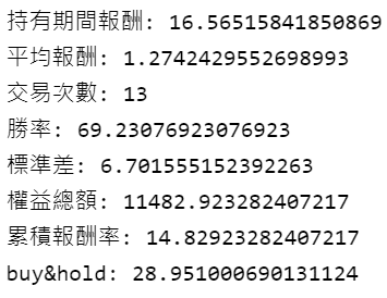
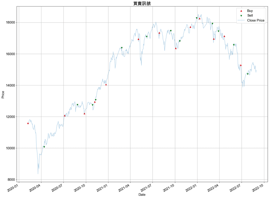
We can find that the cumulative returns are about 16.57%, losing to the buy&hold strategy returns 28.95%. The result of these parameter is not a good idea, so we test the new parameter by optimize method.
buysell(result1,20,20)
The optimize method is check the cumulative returns of different parameters by setting the parameter interval, and select the highest cumulative returns as the optimal parameter.
def optimal(data1,n1:range, n2:range):
    set_0 = 0
    for i in n1:
        for j in n2:
            data =data1.copy()
            buy=[]
            sell=[]
            hold=0
            data['日多ma'] = data['日三線多指標'].rolling(i).mean()
            data['日空ma'] = data['日三線空指標'].rolling(j).mean()
            data.dropna(inplace=True)
            for k in range(len(data)):if  data["日空ma"][k] > data["日多ma"][k]:
                    sell.append(np.nan)
                    if hold !=1:
                        buy.append(data["收盤價"][k])hold = 1
                    else:
                        buy.append(np.nan)
                elif data["日多ma"][k] > data["日空ma"][k]:
                    buy.append(np.nan)
                    if hold !=0:
                        sell.append(data["收盤價"][k])
                        hold = 0
                    else:
                        sell.append(np.nan)
                else:
                    buy.append(np.nan)
                    sell.append(np.nan)
            a=(buy,sell)data['Buy_Signal_Price']=a[0]
            data['Sell_Signal_Price']=a[1]
            data["買賣股數1"]=data['Buy_Signal_Price'].apply(lambda x : 1 if x >0 else 0)
            data["買賣股數2"]=data['Sell_Signal_Price'].apply(lambda x : -1 if x >0 else 0  )
            data["買賣股數"]=data["買賣股數1"]+ data["買賣股數2"]b = data[['Buy_Signal_Price']].dropna()
            c = data[['Sell_Signal_Price']].dropna()
            d = pd.DataFrame(index=c.index, columns = {"Buy_Signal_Price", 'Sell_Signal_Price'})
            for l in range(len(d.index)):
                d["Buy_Signal_Price"][l] = b["Buy_Signal_Price"][l]
                d['Sell_Signal_Price'][l] = c['Sell_Signal_Price'][l]
            d['hold_return'] = (d['Sell_Signal_Price']-d['Buy_Signal_Price'])/d['Buy_Signal_Price']final_equity = 10000
            for m in range(len(d.index)):
                final_equity = final_equity*(d['hold_return'][m]+1)
            cul_ret = ((final_equity-10000)/10000)*100
            if cul_ret>= set_0:
                set_0 = cul_ret
                n1_new = i
                n2_new = j
    return print(' n1:',n1_new,'\n', 'n2:', n2_new,"\n", '累積報酬:', set_0)optimal(result1, n1=range(0,30), n2 =range(0,30) )

The new parameters are used to recalculate the backtesting results and the entry&exit points. The holding period returns are better than buy&hold strategy.
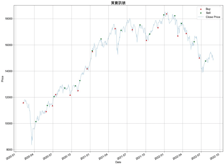
We can see that the SMA cross strategy only have 12.75% cumulative returns, nearly doubling the loss of the buy&hold strategy in the beginning setting parameter. We can find that during the bull market of 2020/4 to 2021/4, our strategy didn’t obtain much of the gains. After optimization, we can see that the cumulative returns are 33.25% and beat the buy&hold strategy. Our strategy also participated in bull market period from 2020/4 to 2021/4, and the win rate is about 67%. But there is something to note:
1. The backtesting results do not take into account the commission fee.
After all, we will introduce others indicators in the future. As a result, if readers are interested in various of trading strategies, welcome to purchase the plan offered in TEJ E-Shop. Construct trading strategies fitting you with high quality database.
Last but not least, please note that “Stocks this article mentions are just for the discussion, please do not consider it to be any recommendations or suggestions for investment or products.” Hence, if you are interested in issues like Creating Trading Strategy , Performance Backtesting , Evidence-based research , welcome to purchase the plans offered in TEJ E Shop and use the well-complete database to find the potential event.