
Table of Contents
在金融市場中,精確的價格預測和有效的交易策略是投資成功的關鍵。本文介紹了一個利用 ADF 檢定(Augmented Dickey-Fuller Test)和 ARIMA-GARCH 模型進行股票價格預測的策略。ADF 檢定用於測試時間序列的平穩性,而 ARIMA-GARCH 模型則結合了自回歸整合移動平均模型(ARIMA)和廣義自回歸條件異方差模型(GARCH),以捕捉股票收益率的波動性。本文詳細描述了策略的實現方法和邏輯,並提供了該策略在實際應用中的潛力。
首先,時間序列是按照時間軸排序,展示歷史數據隨時間變化的資料結構。時間序列模型則利用這種資料結構來分析數據的規律和趨勢,通過建立符合這些特徵的模型來預測未來的走向。
我們先來介紹策略會用到的 ADF 檢定以及 ARIMA-GARCH 模型
ADF 檢定(Augmented Dickey-Fuller Test)是一種用於檢驗時間序列資料是否具有單位根(unit root)的統計方法。單位根存在的話,表示該時間序列是非平穩的,具有隨機漫步的特性。ADF 檢定通過引入滯後差分項來解決自相關問題,從而提高檢定的有效性。檢定的基本假設(零假設)是時間序列存在單位根,即非平穩,而備擇假設則是時間序列沒有單位根,即平穩。進行 ADF 檢定可以幫助分析師判斷是否需要對時間序列進行差分或其他處理以達到平穩性,從而適合進一步的統計分析或建模。
ARIMA-GARCH模型是一種結合 ARIMA(整合移動平均自迴歸模型)和 GARCH(廣義自迴歸條件異方差)模型的混合模型,用於時間序列數據的建模和預測。ARIMA 模型處理數據的均值動態,而 GARCH 模型捕捉數據的波動性。這種結合特別適合於金融數據,因其能同時描述數據的均值和波動聚集特性,從而提供更精確的預測和風險評估。
整合移動平均自迴歸模型(ARIMA)
ARIMA模型是一種基礎的時間序列模型,包含自我迴歸(AR)、差分(Differencing)和移動平均(MA)三個主要參數。
廣義自迴歸條件異方差模型(GARCH)
GARCH 模型是一種用來分析時間序列誤差項的模型,在金融領域主要用於衡量資產或股價的波動性。本文將使用 GARCH 模型檢驗 ARIMA 模型的殘差,進行誤差修正。GARCH 模型的參數與 ARIMA 中的 AR 和 MA 不同,它主要針對的是誤差項和變異數。
初始買入操作:
current_stocks 列表。持續調整持倉:
ban_list 列表。ban_list 列表中的股票,選擇新的高報酬率股票,使持倉數保持在 3 檔。本文使用 Windows 11 並以 VSCode 作為編輯器。
import os
import numpy as np
import pandas as pd
import matplotlib
import warnings
warnings.filterwarnings("ignore")

# tej_key
tej_key = 'your key'
api_base = 'https://api.tej.com.tw'

os.environ['TEJAPI_KEY'] = tej_key
os.environ['TEJAPI_BASE'] = api_base

start='2021-01-01'
end='2023-12-29'
資料期間從 2021-01-01 至 2023–12–29,我們只抓電子類市值前 10 大公司作為我們要預測的股票池,並加入加權報酬指數 IR0001,作為大盤比較。
os.environ['mdate'] = start + ' ' + end
os.environ['ticker'] = ' 2330 2317 2454 2412 2308 2303 3711 3045 2382 3008' + ' ' + 'IR0001'
!zipline ingest -b tquant
Custom Factor 可以讓使用者自行設計所需的客製化因子,於本次案例我們用以處理:
window_length 設置為 91 天,ARIMA-GARCH forecast 的 window_length 設置為 90 天。Pipeline() 提供使用者快速處理多檔標的的量化指標與價量資料的功能,於本次案例我們用以處理:
擷取部分 Pipeline 內容如下:
from zipline.pipeline import Pipeline, CustomFactor
from zipline.pipeline.data import TWEquityPricing
from zipline.TQresearch.tej_pipeline import run_pipeline
from zipline import run_algorithm
from zipline.pipeline import CustomFactor, Pipeline
from zipline.pipeline.filters import StaticAssets
from zipline.api import *

from zipline.data import bundles
bundle_data = bundles.load('tquant')
asset_finder = bundle_data.asset_finder
benchmark_asset = asset_finder.lookup_symbol('IR0001', as_of_date=None)
def make_pipeline():
    return Pipeline(
        columns={
            'open': TWEquityPricing.open.latest,
            'close': TWEquityPricing.close.latest,
            'log_returns':LogReturns(),
            'fc_log_returns': ARIMA_GARCH_Forecast()
        },
        screen=~StaticAssets([benchmark_asset]) # 排除大盤的數據
    )
pipeline = make_pipeline()
result = run_pipeline(pipeline, start, end)
result
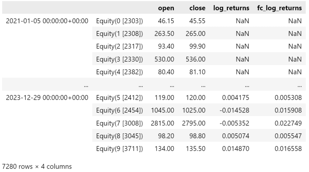
inintialize() 函式用於定義交易開始前的每日交易環境,與此例中我們設置:
context.current_stocks 變數,紀錄持有的股票context.ban_list 變數,紀錄不能買入的股票from zipline.finance import slippage, commission
from zipline.api import set_slippage, set_commission, set_benchmark, attach_pipeline, order_target_percent, symbol, pipeline_output, record, get_datetime, schedule_function, date_rules, time_rules
def initialize(context):
context.current_stocks = []
context.ban_list = set()
set_slippage(slippage.VolumeShareSlippage())
set_commission(commission.PerShare(cost = 0.001425 + 0.003 / 2))
attach_pipeline(make_pipeline(), 'mystrats')
set_benchmark(symbol('IR0001'))
handle_data 函式handle_data() 為構建交易策略的重要函式,會在回測開始後每天被呼叫,主要任務為設定交易策略、下單與紀錄交易資訊。
關於本策略的交易詳細規則請至:ARIMA-GARCH.ipynb
部分程式碼如下:
def handle_data(context, data):
    out_dir = pipeline_output('mystrats')
    # 移除 NaN 值
    out_dir = out_dir.dropna(subset=['fc_log_returns'])

    if not context.current_stocks:
        buy_candidates = out_dir.sort_values(by='fc_log_returns', ascending=False).head(3)

        if buy_candidates.empty:
            print("No stocks selected for initial buying.")
            return

        current_date = get_datetime().strftime('%Y-%m-%d')
        print(f"Initial Rebalance on {current_date}")
        print(f"Initial Buy Candidates:\n{buy_candidates}")

        buy_weight = 1.0 / len(buy_candidates)
        for stock in context.portfolio.positions:
            order_target_percent(stock, 0)
        for i in buy_candidates.index:
            sym = i.symbol
            close = out_dir.loc[i, "close"]
            fc_log_returns = out_dir.loc[i, 'fc_log_returns']

            print(f"Buying {sym} with weight {buy_weight:.2f}")
            order_target_percent(i, buy_weight)

            record(
                **{
                    f'price_{sym}': close,
                    f'fc_log_return_{sym}': fc_log_returns,
                    f'buy_{sym}': True
                }
            )
        context.current_stocks = buy_candidates.index.tolist()
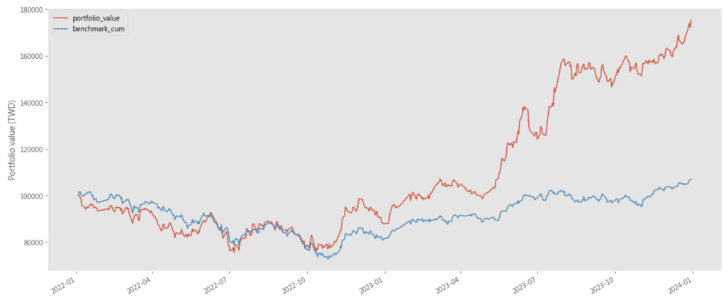
主要用於回測後視覺化策略績效與風險,這裡我們以 matplotlib 繪製投組價值表與 benchmark 價值走勢表
import matplotlib.pyplot as plt

capital_base = 100000  # 設定初始資金

def analyze(context, results):
    plt.style.use('ggplot')
    fig = plt.figure()
    ax1 = fig.add_subplot(111)
    results['benchmark_cum'] = results.benchmark_return.add(1).cumprod() * capital_base
    results[['portfolio_value', 'benchmark_cum']].plot(ax = ax1, label = 'Portfolio Value($)')
    ax1.set_ylabel('Portfolio value (TWD)')

    plt.legend(loc = 'upper left')

    plt.gcf().set_size_inches(18, 8)
    plt.grid()
    plt.show()
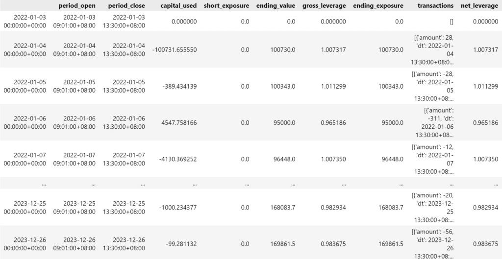
使用 run_algorithm() 執行上述設定的 ARIMA-GARCH 策略,設置交易期間為 start( 2022-01-01 ) 到 end( 2023-12-29 ),使用資料集 tquant,初始資金為十萬元。其中輸出的 results 就是每日績效與交易的明細表。
import pytz
start = pd.Timestamp('2022-01-01', tz=pytz.UTC)
end = pd.Timestamp('2023-12-29', tz=pytz.UTC)

results = run_algorithm(
    start=start,
    end=end,
    initialize=initialize,
    handle_data=handle_data,
    analyze=analyze,
    capital_base=100000,
    data_frequency='daily',
    bundle='tquant'
)
from pyfolio.utils import extract_rets_pos_txn_from_zipline
import pyfolio as pf
# 從 results 資料表中取出 returns, positions & transactions
returns, positions, transactions = extract_rets_pos_txn_from_zipline(results)  # 從 results 資料表中取出 returns, positions & transactions
benchmark_rets = results.benchmark_return  # 取出 benchmark 的報酬率

# 繪製 Pyfolio 中提供的所有圖表
pf.tears.create_full_tear_sheet(returns=returns,
                                     positions=positions,
                                     transactions=transactions,
                                     benchmark_rets=benchmark_rets
                                    )
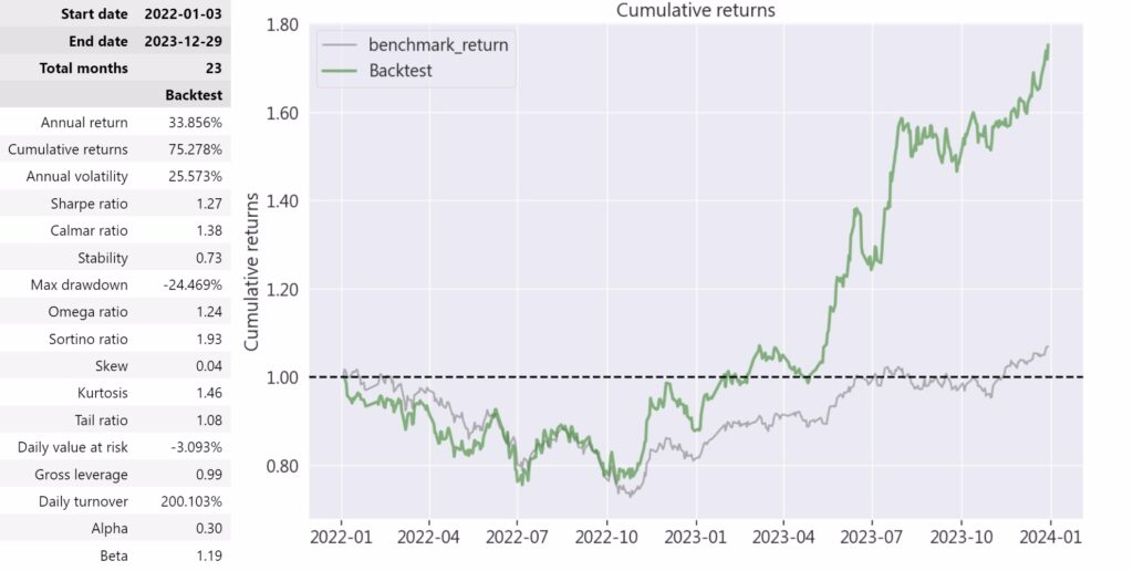
藉由上表我們可以看到 ARIMA-GARCH 策略兩年的年化報酬率達到 33.856%,年化波動度約為 25.573%,另外夏普比率為 1.27,且 α 值為 0.3,顯示 ARIMA-GARCH 策略在相對可控的風險之下,亦能為投資人賺取不俗的超額報酬。因報酬率是用 rolling 的方法,較能適應不同的市場狀況,選股也是透過動態選股的方法,可以抓到比較好的波段進場。在績效比較圖中,可以發現 ARIMA-GARCH 策略於 2023 年後的績效在牛市中明顯較大盤來的好,再次說明本策略優良的獲利以及預測能力。
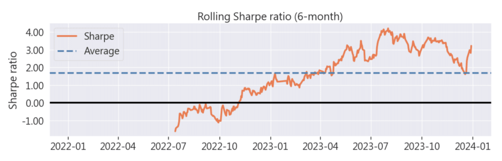
在 Rolling Sharpe ratio 圖中,可以發現此策略表現從 2023 開始才有非常好的表現,可能因為 2022 年大盤市處於熊市的狀況,但儘管如此,此策略的表現在 2022 年還是優於大盤。
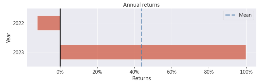
藉由年報酬率圖,我們也可以發現報酬大多來自於 2023 年,完全抵銷了 2022 年的虧損。
本策略在回測期間展示了其獨特的交易邏輯和動態調整機制。通過結合 ADF 檢定和 ARIMA-GARCH 模型進行股票收益率的預測,該策略能夠精確選擇高潛力股票進行投資。策略的動態調整機制允許定期檢查和調整持倉,以應對市場變化和控制風險。這種方法有效地在市場波動中捕捉投資機會,同時保持穩健的風險管理。
總體而言,本策略通過時間序列的波動度模型和靈活的調整機制,展示了其在市場中的應用價值和潛力。未來可以考慮引入更多模型進一步優化策略或是改變模型設定,提升其精準度和整體表現。
溫馨提醒,本次策略與標的僅供參考,不代表任何商品或投資上的建議。之後也會介紹使用 TEJ 資料庫來建構各式指標,並回測指標績效,所以歡迎對各種交易回測有興趣的讀者,選購 TQuant Lab 的相關方案,用高品質的資料庫,建構出適合自己的交易策略。