Apply Financial Data to Predict Stock Price Fluctuation

Table of Contents
Support Vector Machine, short as SVM, is a machine learning algorithm based on Statistics theorem. It is widely used in data classifier and regression. As for this article, we would focus on Classifier.
Simply put, classification of SVM is conducted by draw straight or irregular line(s) to divide different type of data. As for the way to draw the line, we should consider two conditions. First is the degree of difference between data. It is determine by how large the width of the line, briefly speaking. The wider the line, the better to recognize the difference. Second is the Error. Since it is hardly possible to fully distinguish one type of data from the other, we should take error in consideration. The way to measure above conditions is by setting coefficient of error term. As for the weights between them, it requires us to determine.
MacOS & Jupyter Notebook
# Basic
import numpy as np
import pandas as pd# Graph
import matplotlib.pyplot as plt
%matplotlib inline
import seaborn as sns
sns.set()# TEJ API
import tejapi
tejapi.ApiConfig.api_key = 'Your Key'
tejapi.ApiConfig.ignoretz = True
Security Document: Security Types in TAIEX. Code is “TWN/ANPRCSTD”.
Seasonal Financial Table: Seasonally Basic Financial Information. Code is “TWN/EWIFINQ”.
Security Transaction Data Table:Listed securities with unadjusted price and index.Code is “TWN/APRCD”.
Step 1. Filter Security Type
sec_code = tejapi.get('TWN/ANPRCSTD', chinese_column_name = True)condition = (sec_code['上市別'] == 'TSE') & (sec_code['證券種類名稱'] == '普通股')pub_common_stk = sec_code.loc[condition, '證券碼'].to_list()
Select the security type of TSE and consider only common stock.
Step 1. Import Financial Data
fin_data = tejapi.get('TWN/EWIFINQ',
          coid = pub_common_stk,
          mdate= {'gte': '2017-01-01', 'lte': '2021-12-31'},
          opts={'columns': ['coid', 'mdate', 'ac_r103', 'ac_r403']},
          paginate = True,
          chinese_column_name = True)
fin_data = fin_data.dropna()
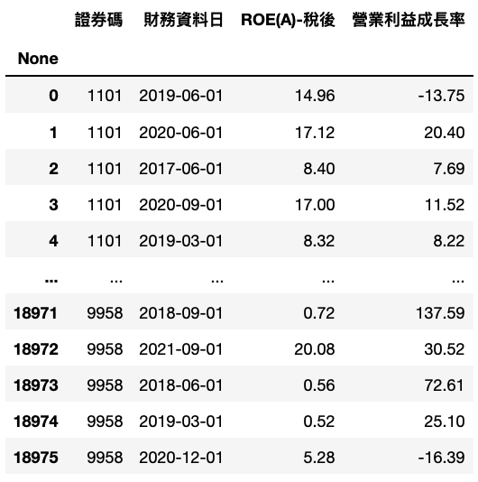
This time, we would apply ROE and Growth of Operating Income Margin. We assume that the larger number of these two indexes represents the better performance.
ROE:Return on Equity, measure one company’s ability of profit
Growth of Operating Income Margin:Operating Income Margin is the proportion of how Operating Income occupy Sales Revenue. As for its growth rate, we apply the index to test whether the company is under stable growth.
The reason we select the above two indexes is that we hope find a balance point between shot-term and mid-term period of investment. This assumption is derive from that we consider ROE is a great measurement for financial performance, but it would easily affected by seasonal rotation and transformation of capital structure. We, therefore, regard Growth of Operating Income Margin as the standard to judge the performance of company management so as to alleviate the shortage of ROE.
Step 3. Import Stock Price & Merge Data
price_df = pd.DataFrame()
for i in pub_common_stk:
    price_data = tejapi.get('TWN/APRCD',
               coid = i,
               mdate= {'gte': '2016-01-01', 'lte': '2021-12-31'},
               opts={'columns': ['coid', 'mdate', 'close_d']},
               paginate = True,
               chinese_column_name = True
               )
    price_df = pd.concat([price_df, price_data], axis = 0)
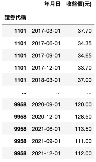
Import Close Price of qualified securities.
def compare(df1, df2):
    df2 = df2.rename(columns = {'證券碼':'證券代碼', '財務資料日':'年月日'})
    compare = pd.merge(df1, df2, how='inner', on=['證券代碼', '年月日'])
    result1 = pd.concat([compare['年月日'], compare['證券代碼']], axis = 1)
    result2 = pd.merge(df1, result1, how='inner', on =['證券代碼', '年月日'])
    return result2ret_df2 = compare(price_df, fin_data)
ret_df2 = ret_df2.set_index(['證券代碼'])
Merge fin_data and price_data, and only keep Date and Price data. We, subsequently, would calculate Holding Period Return between Dates.
Step 4. Calculate Return & Final Data Table
ret_df2['報酬%'] = pd.Series()for i in ret_df2.index.values:
    ret_df2.loc[i]['報酬%'] = pd.Series(ret_df2.loc[i]['收盤價(元)']).pct_change(1)*100
ret_df2 = ret_df2.dropna().reset_index()
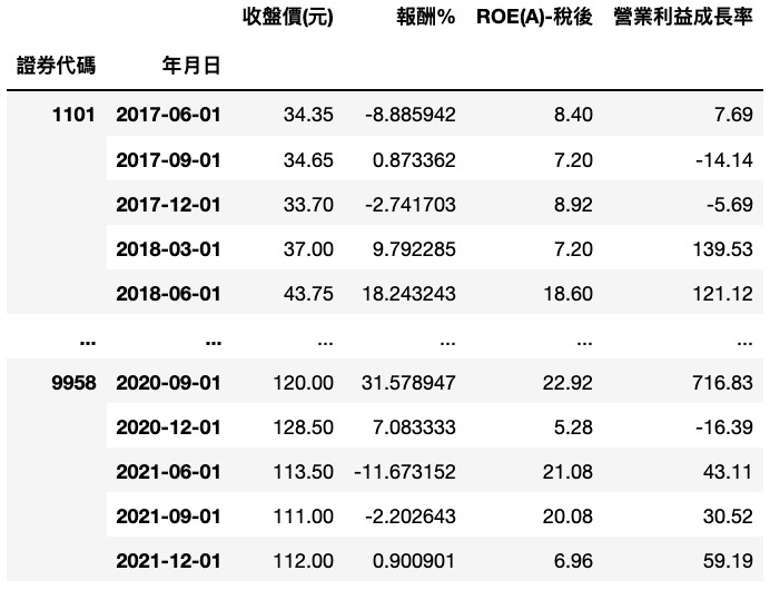
Note:We should import data of each security by loop and calculate return separately so as to avoid the circumstances that compute return with different securities.
def compare2(df1, df2):
    df2 = df2.rename(columns = {'證券碼':'證券代碼', '財務資料日':'年月日'})
    compare = pd.merge(df1, df2, how='inner', on=['證券代碼', '年月日'])
    return comparedata = compare2(ret_df2, fin_data).set_index(['證券代碼','年月日'])
Step 5. Outlier
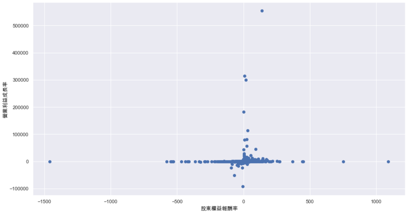
Based on above chart, we can say that outlier problem exists in both ROE and Growth of Operating Income Margin. Hence, we would set the standard of exceeding standard deviation to exclude those outliers.(Considering the length of article, please check complete process in Source Code)
Step 6. Standardize Distribution of Data
import sklearn.preprocessing as preprocessingdata_rmout = data_no.replace([np.inf, -np.inf], np.nan)
data_rmout = data_no.dropna()
data_std = pd.DataFrame(preprocessing.scale(data_no), index = data_no.index, columns = data_no.columns)
plt.figure(figsize=(15,8))
plt.hist(data_std['ROE(A)-稅後'], bins = 50)
plt.hist(data_std['營業利益成長率'], bins = 50, alpha =0.7)
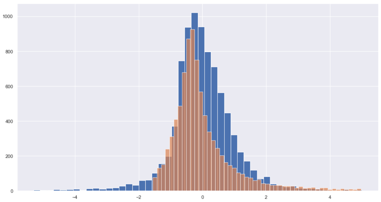
According to above distribution, it is clear that data has been standardized and the distribution of two indexes is similar.
Step 1. Data Split
from sklearn.model_selection import train_test_splitdata_train, data_test = train_test_split(data_std, test_size = 0.2, random_state = 0)
Step 2. Model Fitting
from sklearn.svm import SVCcf = SVC(
C=10.0, break_ties=False, cache_size=200, class_weight=None, coef0=0.0,decision_function_shape='ovr', degree=3, gamma='scale', kernel='linear',max_iter=-1, probability=False, random_state=None, shrinking=True,tol=0.001, verbose=False
)index = ['ROE(A)-稅後', '營業利益成長率']cf.fit(data_train[index], data_train['報酬%'] >  data_train['報酬%'].quantile(0.5))
Checking the setting area of model would know that what we apply is the structure of linear model. To boot, considering that linear may give rise to a too simple model, we set the coefficient of error as 10 so as to increase the complexity of model. As for the standard to measure up or down, we set the standard of “ larger or smaller than median”.
Step 3. Visualize Data Classifier
from mlxtend.plotting import plot_decision_regionsindex_plot = data_test[index].values
labels_plot = (data_test['報酬%'] > data_test['報酬%'].quantile(0.5)).astype(int).valuesplot_decision_regions(index_plot, labels_plot, cf)
plt.xlabel('股東權益報酬率')
plt.ylabel('營業利益成長率')
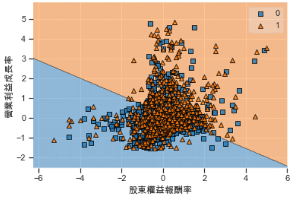
With above chart, model makes us conclude that higher ROE and Growth of Operating Income Margin brings about potential growth, same as our previous assumption.
Step 4. Test Result
# TRAIN
cf.score(data_train[index], data_train['報酬%'] >  data_train['報酬%'].quantile(0.5))# TEST
cf.score(data_test[index], data_test['報酬%'] >  data_test['報酬%'].quantile(0.5))
Train Data Score:0.5857
Valid Data Score:0.5965
The scores are both larger than 0.5, which means that model is effective. On top of that, Valid Data outperforming Train Data represents that there is no overfitting.
This article firstly show you the selection of data and pre-processing. Subsequently, implement model fitting, visualization and train-valid test. The part of process of data processing, we illustrate the meaning of ROE and Growth of Operating Income Margin. If you prefer other indexes, welcome check TEJ Database. During model fitting, we select the simple linear structure so as to make you understand the basic settings of parameters. Lastly, by visualization of model result, we prove that “The larger the indexes, the better the potential”. And, confirm the effectiveness of model by calculating scores of train and valid data.
Last but not least, if you are interested in machine learning, please keep following us. We will publish more articles about other applications. Besides, welcome to purchase the plans offered in TEJ E Shop and use the well-complete database to implement your own model.