We calculate the win rate and return by industry for the emerging market to listed market. As opposed to the company releasing news — the event day study that will apply to the listed market.

Table of Contents
Difficulty: ★★☆☆☆
Advice: This article use Python to select and classify data, then implement the visualization, which required the readers to have the basic knowledge of visualization and programming.
There are some common investment method or trading strategies in investment forums, such as following institutional investors. Today, we would like to explore whether the ‘’sweet period’’ are efficient for trading, or just a fallacy.
Window10 Spyder
import numpy as np
import pandas as pd
import matplotlib.pyplot as plt
plt.rcParams['axes.unicode_minus'] = False
plt.rcParams['font.sans-serif'] = ['Microsoft JhengHei']import tejapi
import time
tejapi.ApiConfig.api_key="YOUR KEY"
tejapi.ApiConfig.ignoretz = True
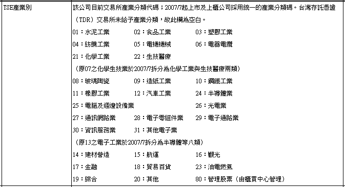
TEJ API company information: Code is (TWN/AIND), ’’TSE industry’’
TEJ PRO database: IPO of newly listed company
The data is taken from the TEJ PRO database and the period is from 1970 to 2022.
df = pd.read_excel('C:/Users/user/Desktop/Tej/PreIPO.xlsx')
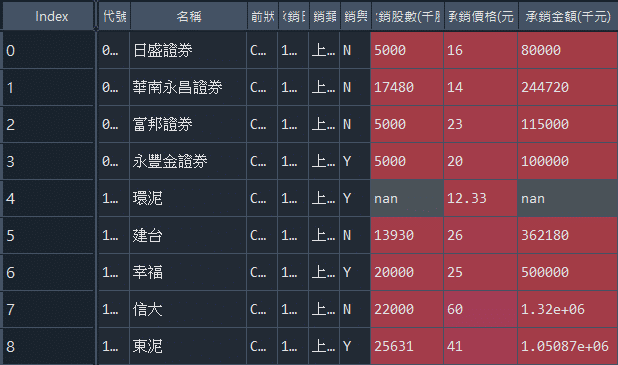
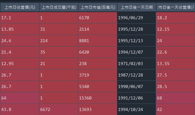
First, select the required data field, then create a Dataframe(A3) to calculate the returns. Finally, rename the field to returns, delete the first day close price and merge the company name and code.
A1 = df[['代號','名稱','上市日收盤價(元)','上市日後一天收盤價(元)','上市日後二天收盤價(元)','上市日後三天收盤價(元)','上市日後四天收盤價(元)','上市日後五天收盤價(元)']]A2 = A1[['上市日收盤價(元)','上市日後一天收盤價(元)','上市日後二天收盤價(元)','上市日後三天收盤價(元)','上市日後四天收盤價(元)','上市日後五天收盤價(元)']]A3 = A2.copy()for i in range(1, len(A2.columns)):
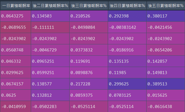
A3.iloc[:,i:i+1] = ((A2.iloc[:,i:i+1].values)/(A2.iloc[:,0:1].values))-1A3 = A3.rename(columns={'上市日後一天收盤價(元)' : '後一日累積報酬率%',
'上市日後二天收盤價(元)' : '後二日累積報酬率%',
'上市日後三天收盤價(元)' : '後三日累積報酬率%',
'上市日後四天收盤價(元)' : '後四日累積報酬率%',
'上市日後五天收盤價(元)' : '後五日累積報酬率%'}, inplace = False)data = A3.drop('上市日收盤價(元)',axis=1)
data1 = A1.join(data, how = "left")
The we make a list with code name to obtain the TEJ API industry, and change the company name to code name, which is convenient for us to merge data. Among them, some special industry must be deleted, because there may be too few sample or special properties is excluded.
Company = A1['代號'].to_list()
Detail = tejapi.get('TWN/AIND', chinese_column_name = True , paginate = True, coid = Company,
                    opts={'columns':['coid','ind1']}) # 舊產業名Detail = Detail.rename(columns={"公司簡稱" : "代號"}, inplace = False)qq = Detail[Detail['TSE 產業別'] != "17" ]
qq = qq[qq['TSE 產業別'] != "14" ]
qq = qq[qq['TSE 產業別'] != "19" ]
qq = qq[qq['TSE 產業別'] != "20" ]
qq = qq[qq['TSE 產業別'] != "80" ]
qq = qq[qq['TSE 產業別'] != "32" ]
qq = qq[qq['TSE 產業別'] != "33" ]
qq = qq[qq['TSE 產業別'] != "34" ]
qq = qq[qq['TSE 產業別'] != "91" ]
Finally, the filtered industry will be combined with the previously calculated returns to obtain the company that we need to successfully listed.
PreIPO = data1.merge(qq, on='代號')
First, we should delete the NA data, and use the industry as a target to calculate the win rate separately. The win rate is that as long as the returns is positive and divided the total company of the industry.
PreIPO = PreIPO.dropna(axis=0,how='any')industry_name = np.unique(PreIPO[['TSE 產業別']])payoff = np.array(['後一日累積報酬率%','後二日累積報酬率%','後三日累積報酬率%','後四日累積報酬率%','後五日累積報酬率%'])industry_number = len(PreIPO.groupby('TSE 產業別').count())save_IPO = list()
for i in range(industry_number):
    for j in range(len(payoff)):
        positive_payoff = len(PreIPO[(PreIPO['TSE 產業別'] == industry_name[i]) & (PreIPO[payoff[j]] > 0)])
        total_number = len(PreIPO[(PreIPO['TSE 產業別'] == industry_name[i])])
        save_IPO.append(f'{round(positive_payoff/total_number*100,2)}')
Next, draw a picture. Read the complete code of the last page for the detail code.
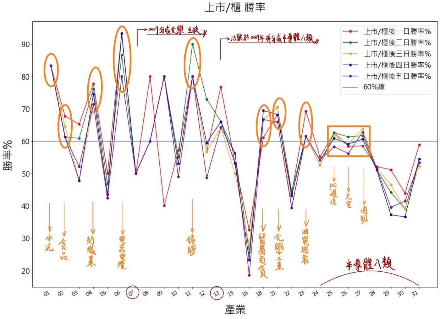
The picture express that the win rate of the industry, because the data will be more difficult to check if we it is displayed in Chinese, it may be squeezed together, so the editor write down the adjustment time. We find that the highest win rate industry is electrical cables. If investors pursue the win rate as efficiency, they can refer the results of this chart.
Next, we calculate the industry average returns.
PreIPO = PreIPO.dropna(axis=0,how='any')industry_name = np.unique(PreIPO[['TSE 產業別']])payoff = np.array(['後一日累積報酬率%','後二日累積報酬率%','後三日累積報酬率%','後四日累積報酬率%','後五日累積報酬率%'])industry_number = len(PreIPO.groupby('TSE 產業別').count())save_IPO = list()for i in range(industry_number):
    for j in range(len(payoff)):
        industry_payoff = PreIPO[payoff[j]][PreIPO['TSE 產業別']==industry_name[i]].mean()save_IPO.append(f'{round(industry_payoff*100,2)}')
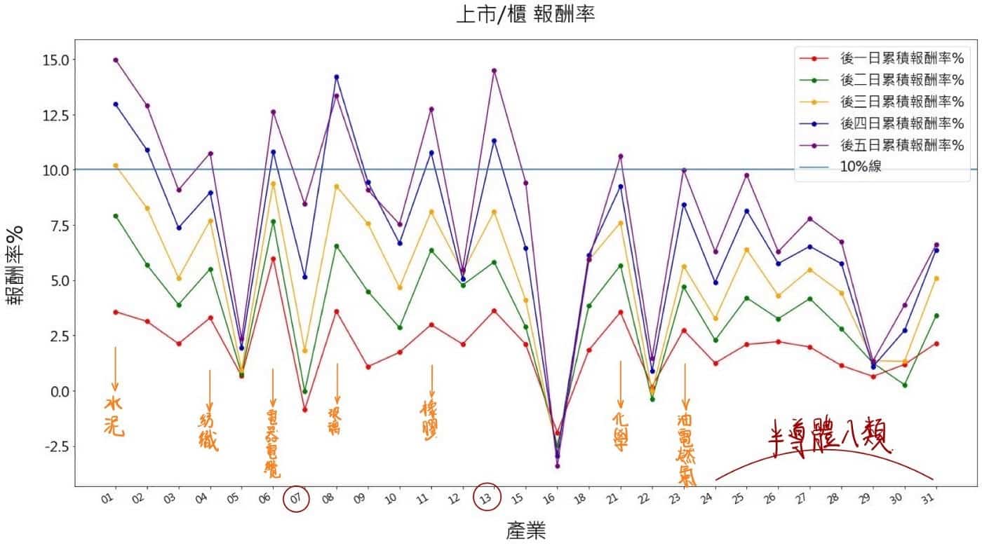
We find that the higher returns depending on the numbers of the days in some industry, and the others fluctuates smaller. In terms of the electrical cables industry with the highest win rate, its win rate is high and the standard deviation is small. However, the rubber industry which the win rate is similar to the electrical cable industry, the volatility is higher than the electrical cable industry.
If we choose to use this investment strategy to carry out short-term operation, we can filter our suitable style. If we want to bear the volatility to obtain returns or maintain the win rate. This article would let readers know that the sweet period is exist, and it can be used to an investment strategy. We also find that the sweet period is not applicable to all industry when we subdivide the industry. It’s still suggested investor to do more analysis, which is less likely to loss in investment.
