Table of Contents
Bollinger Band is a technical indicator that John Bollinger invented in the 1980s. Bollinger Band consists of the concepts of statistics and moving averages. The moving Average(MA) is the average closing price of a past period. Usually, the period of MA in Bollinger Band is 20 days, and Standard Deviation(SD) is usually represented by σ in mathematical sign, which is used to evaluate the data’s degree of discrete.
Bollinger Band is composed of three tracks:
● The upper track:20 MA+double standard deviation
● The middle track:20 MA
● The lower track:20 MA+double standard deviation
The investment target price distribution during the long-term observation period will be Normal Distribution. According to statistics, there is a 95% probability that the price will present between μ − 2σ and μ + 2σ, which is also called a 95% Confidence Interval(CI). Bollinger Band is the technical indicator based on the theories above.
This article uses Windows 11 as a system and jupyter notebook as an editor.
The backtesting time period is between 2021/04/01 to 2022/12/31, and we take AUO(2409), Taiwan’s leading panel manufacturers, as an example in this study.
First, we created Pipeline dunction. Pipeline(), a function in TQuant Lab, enables users to process multiple assets’ trading-related data quickly. In today’s article, we use it to process:
Next, we used Initialize(), a function users can set up the trading environment at the beginning of the backtest period. In this article, we set up :
Pipline() function into backtesting.In addition, we created handle_data() function to process data and make orders daily and obtain the upper, lower, and middle bounds lines for each day’s pipeline.
For visualization, we apply matplotlib.pyplot for observing the trading signals and the portfolio value visualization in our study.
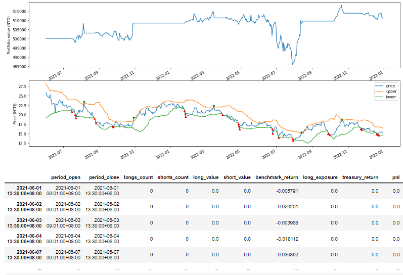
Via run_algorithm(), we can execute the strategy we built above. The backtesting time period is set between 2021-06-01 to 2022-12-31. We assume the initial capital base is 500,000. The output of run_algorithm(), which is results, contains information on daily performance and trading receipts.
By observing the following graph, we can discover that there is an upper trend between 2021/11 to 2021/12. Since the close prices were not able to hit the lower bound, there was no buying transaction in this time period, so that made us fail to earn a profit.
The same issue has happened in the continuously lower trend. A sharp lower trend occurred from 2022-04, which led to consistently touching the lower bound. That means we have bought a bunch of stocks in this time zone. However, after the price recovered shortly, the close price touched the upper bound immediately. As a result, we sell the holding positions and earn a net loss during this time period.
As a matter of fact, due to the latency of 20 days Bollinger band, the band has difficulty reflecting the short-term high volatility price movement. If your target asset is more volatile, we suggested shortening the duration of the Bollinger band or adding trend-related indicators to fine-tune your strategy.
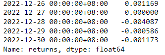
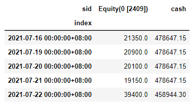
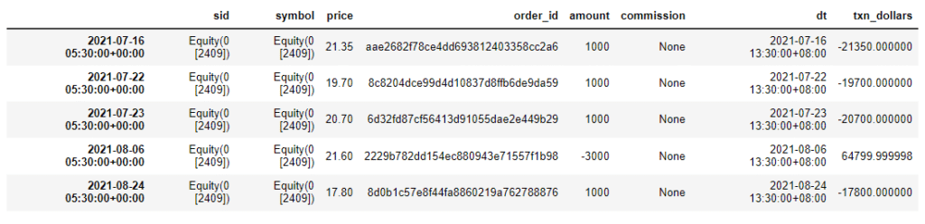
Then, we used Pyfolio module which came with TQuant Lab to analyze strategy’s performance and risk. First, we can calculate returns, positions, and trading records, the following is the results.
Calculating daily portfolio return.
Following is the descriptions of each colums:
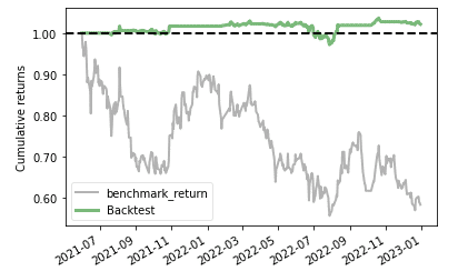
After organized all the data above, we can plot the figure and compare Accumulated Return and Benchmark Return.
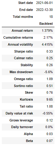
With show_perf_stats() this function, we can easily showcase the performance and risk analysis table.
From late 2021 to 2022, the stock price of AUO is clearly in a downward spiral. if choosing buy and hold strategy, the accumulated return would turn out to be -40% to -50%. On the contrary, with Bollinger band strategy, the performance is way better than the buy and hold strategy.
However, the pure Bollinger Bands strategy tends to have the disadvantage of exiting prematurely during the rebound phase after a significant downward trend and the predicament of entering very rarely during the upward phase. Therefore, for stocks with significant price fluctuations, it is recommended to use other indicators to assess trend strength and optimize their strategy.
Please note that this strategy and the underlying assets are for reference only and do not constitute any recommendations for commodities or investments. In the future, we will also introduce the use of TEJ database to construct various indicators and backtest indicator performance. So, readers interested in various trading backtesting can choose relevant solutions from TEJ Solutions to build their own trading strategies with high-quality databases.
Source Code
Extended Reading
